# packages ----
library(tidycensus)
library(tigris)
library(tidyverse)
library(sf)
library(areal)
library(janitor)
library(here)
library(units)
library(knitr)
library(kableExtra)
library(tmap)
library(patchwork)
library(scales)
library(digest)
library(mapview)
library(biscale)
library(cowplot)
library(glue)
library(ggtext)
library(leafpop)
# conflicts ----
library(conflicted)
conflicts_prefer(dplyr::filter)
# options ----
options(scipen = 999) # turn off scientific notation
options(tigris_use_cache = TRUE) # use data caching for tigris
# reference system ----
## set common projected coordinate reference system used throughout this analysis
crs_projected <- 3310 # see: https://epsg.io/3310Estimating Demographics of Custom Spatial Features
Accessing U.S. Census Bureau Data & Calculating Weighted Averages with Areal- and Population-Weighted Interpolation
1 Background
Note
For comments, suggestions, corrections, or questions on anything below, contact david.altare@waterboards.ca.gov, or open an issue on github.
Warning
This is a draft / work in progress – some parts are still under development, and existing parts may change.
This document provides an example of how to use tools available from the R programming language (R Core Team 2023) to estimate characteristics of any given target spatial area(s) (e.g., neighborhoods, project boundaries, water supplier service areas, etc.) based on data from a source dataset containing the characteristic data of interest (e.g., census data, CalEnviroScreen scores, etc.), especially when the boundaries of the source and target areas overlap but don’t necessarily align with each other. It also provides some brief background on the various types of data available from the U.S Census Bureau, and links to a few places to find more in-depth information.
This particular example estimates demographic characteristics of community water systems in the Sacramento County area (the target dataset). It uses the tidycensus R package (Walker and Herman 2023) to access selected demographic data from the U.S. Census Bureau (the source dataset) for census units whose spatial extent covers those water systems’ service areas, then uses the sf package (Pebesma and Bivand 2023) package (for working with spatial data) and the tidyverse collection of packages (Wickham et al. 2019) (for general data cleaning and transformation) to estimate some demographic characteristics of each water system based on that census data. It also uses the areal R package (Prener et al. 2019) to check some of the results, and as general guidance on the principles and techniques for implementing areal interpolation.
This example is just intended to be a simplified demonstration of a possible workflow. For a real analysis, additional steps and considerations – that may not be covered here – may be needed to deal with data inconsistencies (e.g., missing or incomplete data), required level of precision and acceptable assumptions (e.g. more fine-grained datasets or more sophisticated techniques could be used to estimate/model population distributions), or other project-specific issues that might arise.
2 Setup
The code block below loads required packages for this analysis, and sets some user-defined options and defaults. If they aren’t already installed on your computer, you can install them with the R command install.packages('package-name') (and replace package-name with the name of the package you want to install).
3 Census Data Overview
This section provides some brief background on the various types of data available from the U.S. Census Bureau (for more information about census data available for tribal areas / populations, see Section 12). A later section – Section 5 – demonstrates how to retrieve data from the U.S. Census Bureau using the tidycensus R package. Most of the information covered here comes from the book Analyzing US Census Data: Methods, Maps, and Models in R, which is a great source of information if you’d like more detail about any of the topics below (Walker 2023b).
Note
If you’re already familiar with Census data and want to skip this overview, go directly to the next section: Section 4
Different census products/surveys contain data on different variables, at different geographic scales, over varying periods of time, and with varying levels of certainty. Therefore, there are a number of judgement calls to make when determining which type of census data to use for an analysis – e.g., which data product to use (Decennial Census or American Community Survey), which geographic scale to use (e.g., Block, Block Group, Tract, etc.), what time frame to use, which variables to assess, etc.
More detailed information about U.S. Census Bureau’s data products and other topics mentioned below is available here.
3.1 Census Unit Geography / Hierarchy
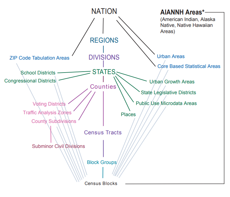
Publicly available datasets from the U.S Census Bureau generally consist of individual survey responses aggregated to defined census units (e.g., census tracts) that cover varying geographic scales. Some of these units are nested and can be neatly aggregated (e.g., each census tract is composed of a collection of block groups, and each block group is composed of a collection of blocks), while other census units are outside this hierarchy (e.g., Zip Code Tabulation Areas don’t coincide with any other census unit). Figure 1 shows the relationship of all of the various census units.
Commonly used census statistical units like tracts and block groups have target population size ranges, and can be adjusted every 10 years (with the decennial census) based on population changes. For example, all ACS 5-year datasets prior to 2020 use the 2010 boundaries for tracts, block groups, and blocks, and all ACS 5-year datasets from 2020 onward (presumably through 2029) use the 2020 boundaries for those units. Census tracts are generally around 4,000 people, with a range from about 1,200 to 8,000, and block groups generally contain 600 to 3,000 people. Blocks are the smallest census units, and are “areas bounded by visible features, such as streets, roads, streams, and railroad tracks, and by nonvisible boundaries, such as selected property lines and city, township, school district, and county limits and short line-of-sight extensions of streets and roads”. For example, a census block may be “a city block bounded on all sides by streets”, while “blocks in suburban and rural areas may be larger, more irregular in shape, and bounded by a variety of features, such as roads, streams, and transmission lines”.
Caution
Census boundaries can change over time. Commonly used statistical units like tracts, block groups, and blocks tend to be revised every 10 years (with the decennial census), so it’s important to use a census boundary dataset that matches the version of the census demographic data you’re retrieving; otherwise, the demographic data may not match geographic areas in your boundary dataset. In some cases, a census unit that exists in a given year of the census data may not exist at all in a different year’s dataset, because census units can be split or merged when boundaries are revised.
For a list of the different geographic units available for each of the different census products/surveys (see Section 3.2) that can be accessed via the tidycensus package, go here.
3.2 Census Datasets / Surveys
The Decennial Census is conducted every 10 years, and is intended to provide a complete count of the US population and assist with political redistricting. As a result, it collects a relatively limited set of basic demographic data, but (should) provide a high degree of precision (i.e., in general it should provide exact counts). It is available for geographic units down to the census block (the smallest census unit available – see Section 3.1). For information about existing and planned future releases of 2020 census data products, go here.
The American Community Survey (ACS) provides a much larger array of demographic information than the Decennial Census, and is updated more frequently. The ACS is based on a sample of the population (rather than a count of the entire population, as in the Decennial Census), so it represents estimated values rather than precise counts; therefore, each data point is available as an estimate (typically labeled with an “E” in census variable codes, which are discussed in Section 3.3 ) along with an associated margin of error (typically labeled with “M” or “MOE” in census variable codes) around its estimated value. The MOEs for ACS data are typically provided at a 90% confidence level – to calculate the 90% confidence interval for an estimate, add the MOE to the estimated value to get the upper bound of the confidence interval, and subtract the MOE from the estimate to get the lower bound of the confidence interval (for more information see here). Note that it’s possible to calculate MOEs for some types of derived estimates of census data, such as aggregating data across multiple census units or calculating proportions and percentages (see here for more information); however, it may be difficult or not possible to calculate MOEs for some more complicated types of derived estimates (like some of the aggregation methods described below).
The ACS is available in two formats. The 5-year ACS is a rolling average of 5 years of data (e.g., the 2021 5-year ACS dataset is an average of the ACS data from 2017 through 2021), and is generally available for geographic units down to the census block group (though some 5-year ACS data may only be available at less granular levels). The 1-year ACS provides data for a single year, and is only available for geographies with population greater than 65,000 (e.g., large cities and counties). Therefore, only the 5-year ACS will be useful for any analysis at a relatively fine scale (e.g., anything that requires data at or more detailed than the census tract level, or any analysis that considers smaller counties/cities – by definition, census tracts always contain significantly fewer than 65,000 people).
In addition to the Decennial Census and ACS data, a number of other census data products/surveys are also available. For example, see the censusapi R package (here or here) for access to over 300 census API endpoints. For historical census data, see the discussion here on using NHGIS, IPUMS, and the ipumsr package.
3.3 Census Variables / Codes
Each census product collects data for many different demographic variables, and each variable is generally associated with an identifier code. In order to access census data programmatically, you often need to know the code associated with each variable of interest. When determining which variables to use, you need to consider what census product contains those variables (see Section 3.2) and how they differ in terms of time frame, precision, spatial granularity (see Section 3.1), etc.
The tidycensus package offers a convenient generic way to search for variables across different census products using the load_variables() function, as described here.
The following websites may also be helpful for exploring the various census data products and finding the variable names and codes they contain:
Census Reporter (for ACS data): https://censusreporter.org/ (especially https://censusreporter.org/topics/table-codes/)
Census Bureau’s list of variable codes, e.g.:
2020 Census codes: https://api.census.gov/data/2020/dec/pl/variables.html
2022 ACS 5 year codes: https://api.census.gov/data/2022/acs/acs5/variables.html
Census Bureau’s data interface (for Decennial Census and ACS, and other census datasets): https://data.census.gov/cedsci/
National Historical Geographic Information System (NHGIS) (for ACS data and historical decennial Census data): https://www.nhgis.org/
4 Target Data Boundaries (Water Systems)
In this section, we’ll get the service area boundaries for Community Water Systems within the Sacramento County area. This will serve as the target dataset – i.e., the set of areas which we’ll be estimating the characteristics of – and will also be used to specify the geographic areas of the census data we want to retrieve. We’ll also get a dataset of county boundaries which overlap the water service areas in this study, which can also help with specifying what census data to access and/or be used to make maps and visualizations.
4.1 Read Water System Data
In this case, we’ll get the water system dataset from a shapefile that’s saved locally, then transform that dataset into a common coordinate reference system for mapping and analysis (which is defined above in the variable crs_projected).
This water system dataset comes from the California Drinking Water System Area Boundaries dataset. For this example, the dataset has been pre-filtered for systems within Sacramento County (by selecting records where the COUNTY field is “SACRAMENTO”) and for Community Water Systems (by selecting records where the STATE_CLAS field is “COMMUNITY”). Some un-needed fields have also been dropped, remaining fields have been re-ordered.
# read from file
water_systems_sac <- st_read(here('02_data_input',
'water_supplier_boundaries_sac',
'System_Area_Boundary_Layer_Sac.shp')) %>%
st_transform(crs_projected) # transform to common coordinate system
# make sure geometry is valid
if (sum(!st_is_valid(water_systems_sac)) > 0) {
water_systems_sac <- st_make_valid(water_systems_sac)
}You can use the glimpse function (below) to take get a sense of what type of information is available in the water system dataset and how it’s structured.
glimpse(water_systems_sac)Rows: 62
Columns: 12
$ WATER_SY_1 <chr> "HOOD WATER MAINTENCE DIST [SWS]", "MC CLELLAN MHP", "MAGNO…
$ WATER_SYST <chr> "CA3400101", "CA3400179", "CA3400130", "CA3400135", "CA3400…
$ GLOBALID <chr> "{36268DB3-9DB2-4305-A85A-2C3A85F20F34}", "{E3BF3C3E-D516-4…
$ BOUNDARY_T <chr> "Water Service Area", "Water Service Area", "Water Service …
$ OWNER_TYPE <chr> "L", "P", "P", "P", "P", "P", "P", "P", "P", "P", "P", "P",…
$ COUNTY <chr> "SACRAMENTO", "SACRAMENTO", "SACRAMENTO", "SACRAMENTO", "SA…
$ REGULATING <chr> "LPA64 - SACRAMENTO COUNTY", "LPA64 - SACRAMENTO COUNTY", "…
$ FEDERAL_CL <chr> "COMMUNITY", "COMMUNITY", "COMMUNITY", "COMMUNITY", "COMMUN…
$ STATE_CLAS <chr> "COMMUNITY", "COMMUNITY", "COMMUNITY", "COMMUNITY", "COMMUN…
$ SERVICE_CO <dbl> 82, 199, 34, 64, 128, 83, 28, 50, 164, 5684, 14798, 115, 33…
$ POPULATION <dbl> 100, 700, 40, 150, 256, 150, 32, 100, 350, 18005, 44928, 20…
$ geometry <GEOMETRY [m]> MULTIPOLYGON (((-131854.3 3..., POLYGON ((-119809.…Note that this dataset already includes a POPULATION variable that indicates the population served by each water system, which was renamed to water_system_population_reported above (note: I’m not exactly how the data in this variable is derived). However, for this analysis we’ll be making our own estimate of the population within each system’s service area based on U.S. Census Bureau data and the spatial representation of the system boundaries. Given the uncertainty in how the reported population data was derived (including potential temporal differences), the population estimates produced here will likely will not exactly match the reported population data; but, the reported population data may serve as a useful check to make sure our estimates are reasonable.
To make the water system data easier to work with, we can make some more descriptive field names (note that while it’s redundant, we’re using the prefix water_system_ for all field names to distinguish data types when joining this data with other datasets later).
water_systems_sac <- water_systems_sac %>%
rename(water_system_name = WATER_SY_1,
water_system_number = WATER_SYST,
water_system_id = GLOBALID,
water_system_boundary_type = BOUNDARY_T,
water_system_owner_type = OWNER_TYPE,
water_system_county = COUNTY,
water_system_regulating_agency = REGULATING,
water_system_federal_class = FEDERAL_CL,
water_system_state_class = STATE_CLAS,
water_system_service_connections = SERVICE_CO,
water_system_population_reported = POPULATION)Here’s a view of the structure of the revised dataset:
glimpse(water_systems_sac)Rows: 62
Columns: 12
$ water_system_name <chr> "HOOD WATER MAINTENCE DIST [SWS]", "M…
$ water_system_number <chr> "CA3400101", "CA3400179", "CA3400130"…
$ water_system_id <chr> "{36268DB3-9DB2-4305-A85A-2C3A85F20F3…
$ water_system_boundary_type <chr> "Water Service Area", "Water Service …
$ water_system_owner_type <chr> "L", "P", "P", "P", "P", "P", "P", "P…
$ water_system_county <chr> "SACRAMENTO", "SACRAMENTO", "SACRAMEN…
$ water_system_regulating_agency <chr> "LPA64 - SACRAMENTO COUNTY", "LPA64 -…
$ water_system_federal_class <chr> "COMMUNITY", "COMMUNITY", "COMMUNITY"…
$ water_system_state_class <chr> "COMMUNITY", "COMMUNITY", "COMMUNITY"…
$ water_system_service_connections <dbl> 82, 199, 34, 64, 128, 83, 28, 50, 164…
$ water_system_population_reported <dbl> 100, 700, 40, 150, 256, 150, 32, 100,…
$ geometry <GEOMETRY [m]> MULTIPOLYGON (((-131854.3 3.…4.1.1 Alternative Data Retrieval Method
Reading in data from a shapefile is shown above because it’s likely one of the more common ways that users will access their target boundary data. However, depending on the dataset, there may be other ways to access the data. For example, the code chunk below demonstrates an alternative – using the arcgislayers package (Parry 2023) – that connects directly to the source dataset (to retrieve the most recent version) and applies the filters needed to reproduce the dataset in the System_Area_Boundary_Layer_Sac.shp file. Also, note that storing data in formats other than the common shapefile format – such as the geopackage format – can have some advantages (for example, see here).
# load arcgislayers package (see: https://r.esri.com/arcgislayers/index.html)
# install.packages('pak') # only needed if the pak package is not already installed
# pak::pkg_install("R-ArcGIS/arcgislayers", dependencies = TRUE)
library(arcgislayers)
# define link to data source
url_feature <- 'https://gispublic.waterboards.ca.gov/portalserver/rest/services/Drinking_Water/California_Drinking_Water_System_Area_Boundaries/FeatureServer/0'
# connect to data source
water_systems_feature_layer <- arc_open(url_feature)
# download and filter data from source
water_systems_sac_alternative <- arc_select(
water_systems_feature_layer,
# apply filters
where = "COUNTY = 'SACRAMENTO' AND STATE_CLASSIFICATION = 'COMMUNITY'",
# select fields
fields = c('WATER_SYSTEM_NAME', 'WATER_SYSTEM_NUMBER', 'GLOBALID',
'BOUNDARY_TYPE', 'OWNER_TYPE_CODE', 'COUNTY',
'REGULATING_AGENCY', 'FEDERAL_CLASSIFICATION',
'STATE_CLASSIFICATION', 'SERVICE_CONNECTIONS', 'POPULATION')) %>%
# transform to common coordinate system
st_transform(crs_projected) %>%
# rename fields
rename(water_system_name = WATER_SYSTEM_NAME,
water_system_number = WATER_SYSTEM_NUMBER,
water_system_id = GLOBALID,
water_system_boundary_type = BOUNDARY_TYPE,
water_system_owner_type = OWNER_TYPE_CODE,
water_system_county = COUNTY,
water_system_regulating_agency = REGULATING_AGENCY,
water_system_federal_class = FEDERAL_CLASSIFICATION,
water_system_state_class = STATE_CLASSIFICATION,
water_system_service_connections = SERVICE_CONNECTIONS,
water_system_population_reported = POPULATION)
# make sure geometry is valid
if (sum(!st_is_valid(water_systems_sac_alternative)) > 0) {
water_systems_sac_alternative <- st_make_valid(water_systems_sac_alternative)
}4.2 Get County Boundaries
When accessing census data using the tidycensus R package as shown below (in Section 5), it’s often useful (though not strictly required) to know which counties overlap the target dataset (note that, even though the dataset is filtered for systems in Sacramento county, there are some systems whose boundaries extend into neighboring counties). County boundaries may also be useful for making maps in later stages of the analysis. You can get a dataset of county boundaries in California from the TIGER dataset, which can be accessed with R using the tigris R package (Walker 2023a).
counties_ca <- counties(state = 'CA',
cb = TRUE) %>% # simplified
st_transform(crs_projected) # transform to common coordinate systemThen, get a list of counties that overlap with the boundaries of the Sacramento area community water systems obtained above.
counties_overlap <- counties_ca %>%
st_filter(water_systems_sac,
.predicate = st_intersects)
counties_list <- counties_overlap %>% pull(NAME)The counties in the counties_list variable are: San Joaquin, Yolo, Placer, Sacramento.
4.3 Plot Target Data
Figure 2 shows the water systems and county boundaries in an interactive map.
mapview(counties_overlap,
alpha.regions = 0,
zcol = 'NAME',
layer.name = 'County',
legend = FALSE) +
mapview(water_systems_sac,
zcol = 'water_system_name',
layer.name = 'Water System',
legend = FALSE)5 Accessing Census Data
The following sections demonstrate how to retrieve census data from the Decennial Census and the ACS using the tidycensus R package.
In order to use the tidycensus R package, you’ll need to obtain a personal API key from the US Census Bureau (which is free and available to anyone) by signing up here: http://api.census.gov/data/key_signup.html. Once you have your API key, you’ll need to register it in R by entering the command census_api_key(key = "YOUR API KEY", install = TRUE) in the console. Note that the install = TRUE argument means that the key is saved for all future R sessions, so you’ll only need to run that command once on your computer (rather than including it in your scripts). Alternatively, you could save your key to an environment variable and retrieve it using Sys.getenv(). Either way will help you avoid the possibility of entering your API key into any scripts that could be shared publicly.
Caution
Because the boundaries of census units (e.g., tracts, block groups, blocks, etc) can change over time, it’s important to make sure that the version (year) of the census data you’re retrieving matches the version of the census boundary dataset you’re using. The methods shown below retrieve the census boundary dataset together with the census demographic data, which ensures that this won’t be a potential problem. However, if you use a different workflow that retrieves the geographic boundaries and demographic data via separate processes, you should ensure that the versions are consistent.
5.1 Create Spatial Filter
Before downloading the census data, we can create an object that can be used to filter our requests to the census API so that they will only return census units that overlap with our target areas (the object will be passed to the filter_by argument of the get_decennial function below). Note that this isn’t strictly necessary (you could also apply the filter after making the API request), but may helpful to speed the query and reduce memory usage, especially in the case of large queries.
Note 1
At the time of this writing, the filter_by argument of the tidycensus get_decennial and get_acs functions is fairly new, and not yet included in the official documentation.
Also, the filter_by argument is optional, and only appears to accept a simple features (sf) object with a single row / feature (e.g., a single water system), and will not accept an sf object with multiple rows / features. The process below attempts to work around this constraint by joining all of the selected water systems into a single multi-part polygon (i.e., an sf object with a single row). However, if you only want to retrieve data for census units that overlap a single target area (e.g., a single water system), you can skip this step.
water_systems_filter <- water_systems_sac %>%
st_union() %>%
st_as_sf()5.2 American Community Survey (ACS) Data
This section retrieves data from the ACS, using the get_acs() function from the tidycensus package. As of this writing, the most recent version of the 5-year ACS data available is the 2018-2022 ACS – it’s set a variable below (note that this variable is used in multiple places throughout this document).
# set year
acs_year <- 2022Next, we define the list of demographic variables we’d like to retrieve tabular data for, by saving the census variables we want in the census_vars_acs object (see Section 3.3 for more information about how to discover variables of interest and find their associated codes). Here we’re providing descriptive names associated with each variable code, which makes the data easier to work with later, but isn’t strictly necessary (i.e., you could just supply the variable codes alone). Note that the use of prefixes (like population_ or households_) and suffixes (like _count) is intentional – those will be used later as part of the calculation process.
# define variables to pull from the ACS
census_vars_acs <- c(
# --- population variables ---
'population_total_count' = 'B01003_001',
'population_hispanic_or_latino_count' = 'B03002_012', # Total Hispanic or Latino
'population_white_count' = 'B03002_003', # White (Not Hispanic or Latino)
'population_black_or_african_american_count' = 'B03002_004', # Black or African American (Not Hispanic or Latino)
'population_native_american_or_alaska_native_count' = 'B03002_005', # American Indian and Alaska Native (Not Hispanic or Latino)
'population_asian_count' = 'B03002_006', # Asian (Not Hispanic or Latino)
'population_pacific_islander_count' = 'B03002_007', # Native Hawaiian and Other Pacific Islander (Not Hispanic or Latino)
'population_other_count' = 'B03002_008', # Some other race (Not Hispanic or Latino)
'population_multiple_count' = 'B03002_009', # Two or more races (Not Hispanic or Latino)
# --- poverty variables ---
'poverty_total_assessed_count' = 'B17021_001', # also available from 'B17020_001' (at the tract level only). Total population for whom poverty status is determined. Poverty status was determined for all people except institutionalized people, people in military group quarters, people in college dormitories, and unrelated individuals under 15 years old. These groups were excluded from the numerator and denominator when calculating poverty rates.
'poverty_below_level_count' = 'B17021_002', # also available from 'B17020_002' (at the tract level only). Population whose income in the past 12 months is below federal poverty level. A family and every individual in it are considered to be in poverty if the family's total income is less than the dollar value of a threshold that varies depending upon size of family, number of children, & age of householder (for 1- & 2- person households). Income is the sum of wage/salary income; net self-employment income; interest/dividends/net rental/royalty income/income from estates & trusts; Social Security/Railroad Retirement income; Supplemental Security Income (SSI); public assistance/welfare payments; retirement/survivor/disability pensions; & all other income.
'poverty_above_level_count' = 'B17021_019', # also available from 'B17020_010' (at the tract level only). Population whose income in the past 12 months is at or above federal poverty level. A family and every individual in it are considered to be in poverty if the family's total income is less than the dollar value of a threshold that varies depending upon size of family, number of children, & age of householder (for 1- & 2- person households). Income is the sum of wage/salary income; net self-employment income; interest/dividends/net rental/royalty income/income from estates & trusts; Social Security/Railroad Retirement income; Supplemental Security Income (SSI); public assistance/welfare payments; retirement/survivor/disability pensions; & all other income.
# --- household variables ---
'households_count' = 'B19001_001', # also available from variable 'B19053_001'. A household includes all the people who occupy a housing unit - a house, an apartment, a mobile home, a group of rooms, or a single room that is occupied. People not living in households are classified as living in group quarters. NOTE: this only includes occupied households (vacant households are not included in most calculations) - to see occupied vs vacant vs total (occupied & vacant), see variables B25002_001, B25002_002, and B25002_003
'average_household_size' = 'B25010_001', # A measure obtained by dividing the number of people living in occupied housing units by the total number of occupied housing units. This measure is rounded to the nearest hundredth.
# --- household income variables ---
'median_household_income' = 'B19013_001', # also available from 'B19019_001' (at the tract level only). Income in the past 12 months is the sum of wage or salary income; net self-employment income; interest, dividends, or net rental or royalty income or income from estates and trusts; Social Security or Railroad Retirement income; Supplemental Security Income (SSI); public assistance or welfare payments; retirement, survivor, or disability pensions; and all other income.
'households_income_below_10k_count' = 'B19001_002', # count of households with income below $10,000
'households_income_10k_15k_count' = 'B19001_003', # count of households with income $10,000 to $15,000
'households_income_15k_20k_count' = 'B19001_004',
'households_income_20k_25k_count' = 'B19001_005',
'households_income_25k_30k_count' = 'B19001_006',
'households_income_30k_35k_count' = 'B19001_007',
'households_income_35k_40k_count' = 'B19001_008',
'households_income_40k_45k_count' = 'B19001_009',
'households_income_45k_50k_count' = 'B19001_010',
'households_income_50k_60k_count' = 'B19001_011',
'households_income_60k_75k_count' = 'B19001_012',
'households_income_75k_100k_count' = 'B19001_013',
'households_income_100k_125k_count' = 'B19001_014',
'households_income_125k_150k_count' = 'B19001_015',
'households_income_150k_200k_count' = 'B19001_016',
'households_income_above_200k_count' = 'B19001_017', # count of households with income above $200,000
# --- housing costs variables (% of household income) ---
# Housing Costs as a Percentage of Household Income in the past 12 months - NOTE: THIS TABLE IS NEW FOR THE 2022 ACS, AND WON'T BE AVAILABLE FOR PREVIOUS YEARS - Table B25140 shows the count of households paying more than 30% of their income towards housing costs broken out by three tenure categories (owned with a mortgage, owned without a mortgage, and rented). The table also shows the number of households paying more than 50% of their income toward housing costs.
# 'households_count' = 'B25140_001',
'households_mortgage_total_count' = 'B25140_002',
'households_mortgage_housing_costs_over30pct_count' = 'B25140_003',
'households_mortgage_housing_costs_over50pct_count' = 'B25140_004',
'households_no_mortgage_total_count' = 'B25140_006',
'households_no_mortgage_housing_costs_over30pct_count' = 'B25140_007',
'households_no_mortgage_housing_costs_over50pct_count' = 'B25140_008',
'households_rent_total_count' = 'B25140_010',
'households_rent_housing_costs_over30pct_count' = 'B25140_011',
'households_rent_housing_costs_over50pct_count' = 'B25140_012',
# --- other income / economic variables ---
'per_capita_income' = 'B19301_001' # note: per capita income by race (at block group level) available in table B19301I
)Now, we can make the data request, using the get_acs function, which accepts several arguments that specify exactly what data to return.
For this example we’re getting data at the ‘Block Group’ level (with the geography = 'block group' argument) for the demographic variables defined above in the census_vars_acs object (which is passed to the variables argument). As noted above, block group-level data is the most granular level of spatial data available from the ACS, and should provide the best results when estimating demographics for areas whose boundaries don’t align with census unit boundaries. However, note that some variables may only be available at less granular spatial scales (like tracts).
In addition to the tabular data associated with the demographic variables in our list, we’ll also get the spatial data – i.e., the boundaries of the census blocks – by setting the geometry = TRUE argument. When we do this, the tabular demographic data is pre-joined to the spatial data for the associated version of the census boundaries, so the API request returns a single dataset with both the spatial and attribute (demographic) data combined.
Note
The tidycensus package generally returns the Census Bureau’s cartographic boundary shapefiles by default (as opposed to the core TIGER/Line shapefiles, which is the default format returned by the tigris R package). The default cartographic boundary shapefiles are pre-clipped to the US coastline, and are smaller/faster to process (alternatively you can use cb = FALSE to get the core TIGER/Line data) (see here). So the default spatial data returned by tidycensus may be somewhat different than the default spatial data returned by the tigris package, but in general I find it’s best to use the default tidycensus spatial data.
However, at the block level tidycensus returns the more detailed core TIGER/Line shapefiles (i.e., they are identical to the default block-level geographic data returned by tigris). In some cases, that may create minor inconsistencies when working with both blocks and block groups and using the default geographies.
We also narrow down the search parameters geographically by specifying the state (with state = 'CA') and counties (county = counties_list) we’re seeking data for, and provide an object to the filter_by argument which filters the data returned so that it only includes census units that overlap with our target areas. Note that the water_systems_filter object supplied to the filter_by argument was created above in Listing 1 (and see Note 1 above for more information about this argument).
Note
Supplying a list of counties may not be strictly necessary, especially in cases where you supply the optional filter_by argument. However, especially when working with granular data like blocks, supplying the county argument seems to greatly speed the API request.
Also, while by default the tidycensus package returns data in long/tidy format, we’re getting the data in wide format for this example (by specifying output = 'wide') because it’ll be easier to work with for the interpolation method described below to estimate demographics for non-census geographies.
# get census data
census_data_acs <- get_acs(geography = 'block group',
state = 'CA',
county = counties_list,
filter_by = water_systems_filter,
year = acs_year,
survey = 'acs5',
variables = census_vars_acs,
output = 'wide', # can be 'wide' or 'tidy'
geometry = TRUE,
cache_table = TRUE) %>%
st_transform(crs_projected) # convert to common coordinate system
# # apply spatial filter to select only the census units overlapping the target area
# ## NOTE: likely only needed if the 'filter_by' argument above is not provided
# census_data_acs <- census_data_acs %>%
# st_filter(water_systems_sac)The output is an sf object (i.e., a dataframe-like object that also includes spatial data), in wide format, where each row represents a census unit, and the each demographic variable is reported in a separate column. Here’s a view of the contents and structure of the 2022 5-year ACS data that’s returned (only the first few fields are shown):
glimpse(census_data_acs[,1:20])Rows: 1,054
Columns: 21
$ GEOID <chr> "060670081451", "06…
$ NAME <chr> "Block Group 1; Cen…
$ population_total_countE <dbl> 1768, 1881, 1098, 2…
$ population_total_countM <dbl> 520, 585, 395, 583,…
$ population_hispanic_or_latino_countE <dbl> 38, 327, 376, 782, …
$ population_hispanic_or_latino_countM <dbl> 59, 298, 280, 315, …
$ population_white_countE <dbl> 1627, 1337, 293, 18…
$ population_white_countM <dbl> 521, 475, 191, 460,…
$ population_black_or_african_american_countE <dbl> 0, 1, 272, 26, 351,…
$ population_black_or_african_american_countM <dbl> 13, 3, 251, 38, 334…
$ population_native_american_or_alaska_native_countE <dbl> 41, 0, 0, 26, 0, 0,…
$ population_native_american_or_alaska_native_countM <dbl> 58, 13, 13, 42, 13,…
$ population_asian_countE <dbl> 45, 0, 105, 58, 144…
$ population_asian_countM <dbl> 71, 13, 116, 66, 18…
$ population_pacific_islander_countE <dbl> 0, 98, 0, 0, 27, 13…
$ population_pacific_islander_countM <dbl> 13, 98, 13, 13, 50,…
$ population_other_countE <dbl> 0, 0, 39, 0, 0, 0, …
$ population_other_countM <dbl> 13, 13, 63, 13, 13,…
$ population_multiple_countE <dbl> 17, 118, 13, 39, 15…
$ population_multiple_countM <dbl> 27, 125, 20, 57, 25…
$ geometry <POLYGON [m]> POLYGON ((-…Note that the dataset that’s returned includes fields corresponding to Margin of Error (MOE) for each variable we’ve requested (these are the fields that end an M – e.g., “population_total_countM”), since, as noted above in Section 3.2 , the ACS is based on a sample of the population and reports estimated values.
For further analysis, we may want to get the statewide data as a baseline for comparison (this could also be done for other scales, like the county level). We can use a similar process to get that data and clean/format it to match the more detailed data obtained above. Note that in this case we’re also using the 5-year ACS (even though the 1-year ACS is also available at the statewide level, and would provide more up-to-date data) so that the statewide data will be directly comparable to the block group level data obtained above.
census_data_acs_state <- get_acs(geography = 'state',
state = 'CA',
year = acs_year,
survey = 'acs5',
variables = census_vars_acs,
output = 'wide', # can be 'wide' or 'tidy'
geometry = TRUE,
cache_table = TRUE) %>%
st_transform(crs_projected) %>% # convert to common coordinate system
select(-matches('M$')) %>% # the $ specifies "ends with"
# clean names (note this is a little different than the way we renamed fields above, either works)
rename_with(.fn = ~ str_remove(., # remove 'E' (estimate) from field names
pattern = 'E$')) %>%
rename_with(.fn = ~ str_replace(., # add 'E' back to NAME field
pattern = 'NAM',
replacement = 'NAME'))5.3 Decennial Census Data
To get data from the Decennial Census, you can use the get_decennial function, which is very similar to the get_acs() function used above. As of this writing, the most recent version of the decennial census data available is from 2020 (set as a variable below).
# set year
decennial_year <- 2020However, since ACS data contains data on a much broader set of socioeconomic metrics than the Decennial Census, the requested data includes a greatly reduced list of variables, defined in the census_vars_decennial object (see Section 3.3 for more information about how to discover variables of interest and find their associated codes). As above, we’ll provide descriptive names associated with each variable code, which makes the data easier to work with later, but isn’t strictly necessary (i.e., you could just supply the variable codes alone).
# define variables to pull from the decennial census
census_vars_decennial <- c(
'population_total_count' = 'P2_001N',
'population_hispanic_or_latino_count' = 'P2_002N', # Total Hispanic or Latino
'population_white_count' = 'P2_005N', # White (Not Hispanic or Latino)
'population_black_or_african_american_count' = 'P2_006N', # Black or African American (Not Hispanic or Latino)
'population_native_american_or_alaska_native_count' = 'P2_007N', # American Indian and Alaska Native (Not Hispanic or Latino)
'population_asian_count' = 'P2_008N', # Asian (Not Hispanic or Latino)
'population_pacific_islander_count' = 'P2_009N', # Native Hawaiian and Other Pacific Islander (Not Hispanic or Latino)
'population_other_count' = 'P2_010N', # Some other race (Not Hispanic or Latino)
'population_multiple_count' = 'P2_011N', # Two or more races (Not Hispanic or Latino)
'households_count' = 'H1_002N' # households (occupied)
)Next we can make the data request, using the get_decennial function, which is very similar to the get_acs function described above (Section 5.2). However, for this example we’re getting data at the ‘Block’ level (with the geography = 'block' argument) for the demographic variables defined above in the census_vars_decennial object (which is passed to the variables argument). As noted above, block-level data is the most granular level of spatial data available, and should provide the best results when estimating demographics for areas whose boundaries don’t align with census unit boundaries. However, depending on the use case, it may require too much time and computational resources to use the most granular spatial data, and may not be necessary to obtain a reasonable estimate. Also, keep in mind that block-level data may not be available for all variables, and some variables may only be available at less granular spatial scales (like block groups or tracts).
Also note that the water_systems_filter object supplied to the filter_by argument was created above in Listing 1 (and see Note 1 above for more information about this argument).
# get census data
census_data_decennial <- get_decennial(geography = 'block', # can be 'block', 'block group', 'tract', 'county', etc.
state = 'CA',
county = counties_list,
filter_by = water_systems_filter,
year = decennial_year,
variables = census_vars_decennial,
output = 'wide', # can be 'wide' or 'tidy'
geometry = TRUE,
cache_table = TRUE) %>%
st_transform(crs_projected) # convert to common coordinate system
# apply spatial filter to select only the census units overlapping the target area
## NOTE: at detailed (block) level this may be needed - the water_systems_filter
## object may not filter out all blocks (these appear to be blocks that
## border / touch the filter area, but don't overlap with it) - filtering these
## out may avoid complications in subsequent calculations
census_data_decennial <- census_data_decennial %>%
st_filter(water_systems_sac)As above, the output is an sf object (i.e., a dataframe-like object that also includes spatial data), in wide format, where each row represents a census unit, and the population of each racial/ethnic group is reported in a separate column. Here’s a view of the contents and structure of the Decennial Census data that’s returned:
glimpse(census_data_decennial)Rows: 17,721
Columns: 13
$ GEOID <chr> "060670019003011", "…
$ NAME <chr> "Block 3011, Block G…
$ population_total_count <dbl> 53, 20, 181, 100, 12…
$ population_hispanic_or_latino_count <dbl> 4, 6, 8, 11, 1, 14, …
$ population_white_count <dbl> 20, 4, 167, 70, 86, …
$ population_black_or_african_american_count <dbl> 2, 2, 0, 8, 9, 18, 0…
$ population_native_american_or_alaska_native_count <dbl> 0, 0, 0, 0, 0, 0, 0,…
$ population_asian_count <dbl> 19, 5, 2, 1, 23, 8, …
$ population_pacific_islander_count <dbl> 0, 0, 0, 0, 0, 0, 0,…
$ population_other_count <dbl> 0, 0, 0, 0, 0, 0, 0,…
$ population_multiple_count <dbl> 8, 3, 4, 10, 5, 10, …
$ households_count <dbl> 19, 7, 64, 48, 60, 1…
$ geometry <POLYGON [m]> POLYGON ((-1…5.4 Plot Census & Supplier Data
system_plot <- 'SACRAMENTO SUBURBAN WATER DISTRICT'Figure 3 shows the 2022 5-year ACS census units that overlap with one of the water systems (Sacramento Suburban Water District) that we’ll compute demographics for below (note that a single system is shown because plotting the census units that overlap all systems tends to be slow in this format; to view the census boundaries overlapping all systems see Figure 5).
mapview(water_systems_sac %>%
filter(water_system_name == system_plot),
zcol = 'water_system_name',
layer.name = 'Water System',
legend = FALSE) +
mapview(census_data_acs %>%
st_filter(water_systems_sac %>%
filter(water_system_name == system_plot)),
alpha.regions = 0,
color = 'cyan',
lwd = 1.3, label = 'NAME',
layer.name = 'ACS Data',
legend = FALSE) # zcol = 'NAME'6 Compute Water System Demographics
Now we can perform calculations to estimate demographic characteristics for our target areas (water system service boundaries in the Sacramento County area) from our source demographic dataset (census data). For this example, we’ll use the 2022 5-year ACS data that was retrieved above (which is saved in the census_data_acs variable) as our source of demographic data, and we’ll estimate the following for each water system’s service area:
- Total population and population of each racial/ethnic group (using the racial/ethnic categories defined in the census dataset), and each racial/ethnic group’s portion of the total service area population
- Socioeconomic variables like poverty rate, median household income, income distributions, per capita income, and average household size
6.1 Considerations and Alternatives
There are multiple ways this estimation can be done. Which option to pick may depend on multiple factors, such as:
- Level of precision required (higher precision may require more detailed methods)
- Level of certainty in the target area boundaries (higher uncertainty in target area boundaries may make more detailed methods irrelevant/unnecessary)
- Relative size of the target areas to available types of census units (if target areas are relatively large, the results may not be very sensitive to the method chosen, but results for smaller areas may be highly sensitive to choice of method)
- Degree to which the methodology should easily explainable / interpretable (detailed methods may be hard to explain concisely)
- Types of census variables needed (some variables may not be available at certain levels of spatial granularity)
Methods described in this document include the following (in no particular order):
Multi-step process that uses areal interpolation to estimate count variables for the target areas (water systems) from overlapping census units, then uses that estimated count data to make weighted average estimates for remaining variables. See Section 6.2.
Simplified method which uses entire census units that overlap the target areas (water systems) to estimate demographics for those areas. This method is relatively simple and explainable, and makes it possible to produce MOEs for the derived estimates. However, it uses entire census units as proxies for water system service area boundaries, so may produce significantly less precise estimates than other approaches in some cases. See Section 9.1.
Population weighted areal interpolation, using the
interpolate_pwfunction from thetidycensusR package, which implements an approach that is based on Esri’s data apportionment algorithm (see here and here. This attempts to take into account the distribution of the population within census units, by using data from a third more granular dataset as weights for the interpolation process between the source and target areas. This approach likely will produce more precise estimates than the approaches described above, especially for mid- and smaller- sized target areas that may only overlap portions of a relatively small number of census units. However it doesn’t appear to be applicable for very small target areas (small water systems), and doesn’t provide estimates for those areas – more research may be needed on considerations for its use in certain cases. It may also be somewhat difficult to explain the methodology and/or interpret the results. See Section 9.2.Modified version of population weighted areal interpolation, which is somewhat similar to the approach above in that it uses data from a third (more granular) dataset to estimate the distribution of the population within census units (block groups) and determine what portion of each census unit to apply to each target area (water system). This modified approach may especially improve estimates in cases where the target areas (water systems) only overlap a portion of the source data (census units), and may provide somewhat more valid estimates for mid- and smaller- sized water systems (though it still won’t work for very small areas/ systems). However, it may be somewhat complicated for some use cases, may not meaningfully improve estimates for some (mostly larger) systems, and may be somewhat difficult to describe and interpret. See Section 9.3.
In addition, Section 10 describes how to use block level data from the decennial census to produce more detailed population / household count estimates alone.
For simplicity, we’ll apply the first method here, and then save and explore / visualize the results obtained from that method in more detail. However, those results could simply be replaced with the results from any of those other methods described later in Section 9 (or other methods not described in this document).
6.2 Method Overview
This method will employ a multi-step approach:
Estimate values for count-based variables (typically referred to as ‘extensive’ data types) – e.g., total population, population by race/ethnicity, population above / below poverty rate, households by income bracket, etc. – for overlapping census units, using areal interpolation. This is essentially an area-weighted average, which estimates how much of each source unit’s (census unit) count applies to the target area (a given water service area), based on the portion of its area that overlaps that target area. For example, for a census unit that partially overlaps a service area, only a fraction of its count for a given variable will be applied to that service area; for a census unit that completely overlaps a service area, the full count for that variable will be applied to the service area.
For more information about this process and discussion of its use cases, see this journal article, and/or the documentation here and here from the
arealR package.The major simplifying assumption of this approach is that the population or other count-based variable of interest is evenly distributed within each unit in the source data. For example, in this case we’re assuming that population (including the total population and the population of each racial/ethic group), households of each income bracket, populations above / below the poverty rate, etc. are evenly distributed within each census block group.
Note
While this section uses the block group-level count data from the 5-year ACS, there may be cases where it could be useful or necessary to use more granular block-level population data from the decennial census to estimate population densities and distributions within block groups. This could especially be the case when estimating characteristics for small and/or rural areas. See Section 9.2 and Section 9.3 for approaches which implement methods that do that, and Section 10 for detailed estimates of population alone using block-level decennial data.
Also see Section 11 for more information about challenges estimating values for small / rural areas.
- Using the estimated count data (populations, households, etc), compute weighted values for remaining variables, with the associated count data as a weighting factors – e.g., population-weighted values for population based data, or household-weighted values for household-based data. These variables are typically referred to as ‘intensive’ variables.
Note
Although it’s possible to use simple areal interpolation to aggregate these ‘intensive’ variables as well, the multi-step approach described here can be useful because we know (from the population / household count data) that population densities differ between census units. Since we have a reasonable estimate of the count data (population, households, etc.) within each census unit, using a population- or household-weighted average likely will yield more accurate results than a simple area-weighted average for these variables. For example, for per capita income, an area-weighted average would likely over-weight large census areas with lower population densities, and would likely be less meaningful than a population-weighted average.
Areal interpolation of intensive variables may be more useful for cases where we generally have no other information about how density varies between the source polygons.
Some of those considerations are discussed here. More research / input may be needed on this issue.
- Aggregate interpolated values at the water system level, summing the count data for variables computed in step 1, and computing weighted means for count-weighted variables computed in step 2.
6.3 Prepare Census Data
Note that we already transformed the 2022 5-year ACS dataset into the common projected coordinate reference system used for this example immediately after we downloaded the data using the get_acs() function (see Listing 2). This allows us to work with the water system data and the census data together in a common coordinate system.
Before calculating demographics for the target areas, we can do a bit of additional transformation to prepare the census data. First, because we won’t be incorporating the margin of error (MOE) into the analysis below, we can drop them for this example, then clean up the field names.
Tip
It is possible to calculate MOEs for derived estimates – e.g., when aggregating groups of census units – and in many cases it may be worthwhile to do that to provide extra context to the data. However, it may not be possible (or may be very difficult) to calculate MOEs for data estimated using more complex aggregations, such as the areal interpolation shown below – more research on that may be needed.
For guidance on how calculate MOEs for some types of derived estimates, see this document.
For an alternative, simplified approach to estimating census demographics for target areas which includes MOEs for the derived estimates, see Section 9.1.
# drop MOE fields
census_data_acs <- census_data_acs %>%
select(-matches('M$')) # the $ specifies "ends with"
# clean names
names(census_data_acs) <- names(census_data_acs) %>%
str_remove('E$') %>% # remove 'E' (estimate) from field names
str_replace('NAM', 'NAME') # add 'E' back to NAME fieldHere’s a view of the contents and structure of the revised 2022 5-year ACS dataset (only the first few fields are shown):
glimpse(census_data_acs[,1:20])Rows: 1,054
Columns: 21
$ GEOID <chr> "060670081451", "060…
$ NAME <chr> "Block Group 1; Cens…
$ population_total_count <dbl> 1768, 1881, 1098, 27…
$ population_hispanic_or_latino_count <dbl> 38, 327, 376, 782, 3…
$ population_white_count <dbl> 1627, 1337, 293, 181…
$ population_black_or_african_american_count <dbl> 0, 1, 272, 26, 351, …
$ population_native_american_or_alaska_native_count <dbl> 41, 0, 0, 26, 0, 0, …
$ population_asian_count <dbl> 45, 0, 105, 58, 144,…
$ population_pacific_islander_count <dbl> 0, 98, 0, 0, 27, 13,…
$ population_other_count <dbl> 0, 0, 39, 0, 0, 0, 0…
$ population_multiple_count <dbl> 17, 118, 13, 39, 15,…
$ poverty_total_assessed_count <dbl> 1768, 1847, 1098, 27…
$ poverty_below_level_count <dbl> 101, 328, 272, 116, …
$ poverty_above_level_count <dbl> 1667, 1519, 826, 263…
$ households_count <dbl> 680, 718, 405, 905, …
$ average_household_size <dbl> 2.59, 2.62, 2.71, 2.…
$ median_household_income <dbl> 123500, 66768, 56216…
$ households_income_below_10k_count <dbl> 18, 47, 10, 22, 6, 1…
$ households_income_10k_15k_count <dbl> 0, 0, 24, 0, 15, 231…
$ households_income_15k_20k_count <dbl> 0, 13, 18, 0, 51, 12…
$ geometry <POLYGON [m]> POLYGON ((-1…We can also do some other transformations – for example, we can calculate the poverty rate for each census unit (which may be useful for presenting results later).
census_data_acs <- census_data_acs %>%
mutate(poverty_rate_pct_calc_census_unit = case_when(
poverty_total_assessed_count == 0 ~ 0,
.default = 100 * poverty_below_level_count / poverty_total_assessed_count
),
.after = poverty_above_level_count)6.4 Interpolation Step 1: Estimate Data for Count (Extensive) Variables with Areal Interpolation
There are a couple of ways to implement the areal interpolation method. The example below ‘manually’ implements the process using functions from the sf package, for reasons described below. However, note that there are R packages which make it possible to perform areal interpolation with a single function - for example, the sf package’s st_interpolate_aw function and the areal package’s aw_interpolate function. This example uses a more ‘manual’ approach because this makes it possible to use the multi-step process described above, and also produces useful intermediate calculated data for mapping and visualization. However, we can use the single-function approach to double check our implementation of the areal interpolation approach for the count data (see Section 8.1).
Warning
Areal interpolation may not work well in some cases (for example, in areas that are largely rural or near uninhabited areas) In these cases, it’s possible to use more granular block-level population data from the decennial census to estimate population densities and distributions within block groups. See Section 9.2 and Section 9.3 for approaches that implement methods for doing that.
First, clip the census data to the water system boundaries:
census_data_clip <- census_data_acs %>%
mutate(census_unit_area = st_area(.)) %>%
st_intersection(water_systems_sac) %>%
mutate(clipped_area = st_area(.)) %>%
mutate(areal_weight_factor = drop_units(clipped_area / census_unit_area))Figure 4 shows a plot of the census units clipped to the Sacramento Suburban Water District water system, along with the original/complete census units. Note that you can toggle layers on and off (and change their order of appearance) using the layers button in the upper left part of the map (below the zoom buttons).
mapview(water_systems_sac %>%
filter(water_system_name == system_plot),
zcol = 'water_system_name',
layer.name = 'Water System',
legend = FALSE) +
mapview(census_data_acs %>%
st_filter(water_systems_sac %>%
filter(water_system_name == system_plot)),
alpha.regions = 0.15,
col.regions = 'grey',
color = 'black',
lwd = 1,
label = 'NAME',
layer.name = 'ACS Data Full',
legend = FALSE) +
mapview(census_data_clip %>%
filter(water_system_name == system_plot),
alpha.regions = 0,
color = 'cyan',
lwd = 1.3,
label = 'NAME',
layer.name = 'ACS Data Clipped',
legend = FALSE)Next, compute the area-weighted counts for the portions of census units that overlap each water system boundary:
census_data_interpolate <- census_data_clip %>%
mutate(
across(
.cols = ends_with('_count'),
.fns = ~ .x * areal_weight_factor
)) 6.5 Interpolation Step 2: Estimate Weighted Values for Remaining (Intensive) Variables Based on Interpolated Counts
Next, compute weighted values for remaining variables, using estimated count data from the previous step (population or households) as weighting factors:
census_data_interpolate <- census_data_interpolate %>%
mutate(average_household_size_weighted = average_household_size * households_count,
median_household_income_weighted = median_household_income * households_count,
per_capita_income_weighted = per_capita_income * population_total_count)
Caution 1
To calculate an aggregated value for a variable like median household income, which depends on the distribution of the underling data, it may be worth considering whether a weighed average value is an appropriate measure. In some cases, it may be more appropriate to use the counts in each income bracket to estimate a median income, and/or present the income distribution rather than a single value.
For a discussion of the problem and a proposed solution, see this document.
6.6 Interpolation Step 3: Aggregate by Water System
Next, combine the weighted values calculated above to produce the estimates for each water system. We can do this by summing all of the count-based variables computed in step 1 above using areal interpolation, and calculating weighted means for all count-weighted variables computed in step 2 above.
Note that we have to first calculate the denominator for each variable calculated with count-weighted interpolation, because some of those variables contain missing values for records where the denominator is present (and if we don’t remove the missing values, we get an NA for any water system that contains a block group with a missing value for that variable). For example, there are block groups where the median household income is missing, but the total household count is available for that block group – in that case, the weighted average should not include the households in that block group in the denominator; otherwise, the true value will be underestimated.
# aggregate ----
water_system_demographics <- census_data_interpolate %>%
mutate(
average_household_size_denominator = if_else(
is.na(average_household_size),
0,
households_count),
median_household_income_denominator = if_else(
is.na(median_household_income),
0,
households_count),
per_capita_income_denominator = if_else(
is.na(per_capita_income),
0,
population_total_count)
) %>%
group_by(water_system_name) %>%
summarize(
across(
.cols = ends_with('_count'),
.fns = ~ sum(.x)
),
average_household_size_hh_weighted =
sum(average_household_size_weighted, na.rm = TRUE) /
sum(average_household_size_denominator),
median_household_income_hh_weighted =
sum(median_household_income_weighted, na.rm = TRUE) /
sum(median_household_income_denominator),
per_capita_income_pop_weighted =
sum(per_capita_income_weighted, na.rm = TRUE) /
sum(per_capita_income_denominator)
) %>%
ungroup()
# round count data to nearest whole number ----
water_system_demographics <- water_system_demographics %>%
mutate(
across(
.cols = ends_with('_count'),
.fns = ~ round(.x, 0)
))
# glimpse(water_system_demographics_acs_estimated_blocks)
# if population / household counts are zero, set population / household weighted means values to NA ----
water_system_demographics <- water_system_demographics %>%
mutate(
average_household_size_hh_weighted = case_when(
households_count == 0 ~ NA,
.default = average_household_size_hh_weighted
),
median_household_income_hh_weighted = case_when(
households_count == 0 ~ NA,
.default = median_household_income_hh_weighted
),
per_capita_income_pop_weighted = case_when(
population_total_count == 0 ~ NA,
.default = per_capita_income_pop_weighted
)
)Since computing a weighted mean for the median household income may be somewhat inaccurate (as noted above in Caution 1), it may also be worth calculating a grouped median household income based on the income bracket data:
# TO DO: Compute grouped median incomesUsing the aggregated data, we can also compute some additional metrics for each system, like ethnic/racial group portions, poverty rates, income distributions, etc.:
# race / ethnicity ----
water_system_demographics <- water_system_demographics %>%
mutate(
across(
.cols = starts_with('population_'),
.fns = ~ ifelse(population_total_count == 0,
NA,
round(.x / population_total_count * 100, 2)),
.names = "{str_replace(.col, '_count', '_percent')}"
),
.after = population_multiple_count) %>%
select(-population_total_percent) # this always equals 1, not needed
# poverty rate ----
water_system_demographics <- water_system_demographics %>%
mutate(poverty_rate_percent = case_when(
population_total_count == 0 ~ NA,
poverty_total_assessed_count == 0 ~ 0,
.default = 100 * poverty_below_level_count / poverty_total_assessed_count
),
.after = poverty_above_level_count)
# consistent income brackets ----
## 25k brackets ----
water_system_demographics <- water_system_demographics %>%
mutate(households_income_25k_brackets_0_25k_count =
households_income_below_10k_count +
households_income_10k_15k_count +
households_income_15k_20k_count +
households_income_20k_25k_count,
households_income_25k_brackets_25k_50k_count =
households_income_25k_30k_count +
households_income_30k_35k_count +
households_income_35k_40k_count +
households_income_40k_45k_count +
households_income_45k_50k_count,
households_income_25k_brackets_50k_75k_count =
households_income_50k_60k_count +
households_income_60k_75k_count,
.after = households_income_above_200k_count
) # note: above 75k is already in 25k increments
## 50k brackets ----
water_system_demographics <- water_system_demographics %>%
mutate(households_income_50k_brackets_0_50k_count =
households_income_below_10k_count +
households_income_10k_15k_count +
households_income_15k_20k_count +
households_income_20k_25k_count +
households_income_25k_30k_count +
households_income_30k_35k_count +
households_income_35k_40k_count +
households_income_40k_45k_count +
households_income_45k_50k_count,
households_income_50k_brackets_50k_100k_count =
households_income_50k_60k_count +
households_income_60k_75k_count +
households_income_75k_100k_count,
households_income_50k_brackets_100k_150k_count =
households_income_100k_125k_count +
households_income_125k_150k_count,
.after = households_income_25k_brackets_50k_75k_count
) # note: above 150k is already in 50k increments
# portion of households paying more than 30% / 50% of income on housing ----
water_system_demographics <- water_system_demographics %>%
mutate(households_all_housing_costs_over30pct_percent =
ifelse(households_count == 0,
NA,
100 * (households_mortgage_housing_costs_over30pct_count +
households_no_mortgage_housing_costs_over30pct_count +
households_rent_housing_costs_over30pct_count) /
households_count),
.after = households_rent_housing_costs_over50pct_count) %>%
mutate(households_all_housing_costs_over50pct_percent =
ifelse(households_count == 0,
NA,
100 * (households_mortgage_housing_costs_over50pct_count +
households_no_mortgage_housing_costs_over50pct_count +
households_rent_housing_costs_over50pct_count) /
households_count
),
.after = households_all_housing_costs_over30pct_percent)
# round values ----
water_system_demographics <- water_system_demographics %>%
mutate(
across(
.cols = ends_with('_count'),
.fns = ~ round(.x, 0)
)) %>%
mutate(
across(
.cols = ends_with('_percent'),
.fns = ~ round(.x, 2)
))6.7 View Results
We now have a dataset with the selected metrics from the census data (source data) estimated for each of the water system service areas (target geographic features). Here’s a view of the contents and structure of the re-formatted dataset (only the first few fields are shown):
glimpse(water_system_demographics[,1:20])Rows: 62
Columns: 21
$ water_system_name <chr> "B & W RESORT MARI…
$ population_total_count <dbl> 0, 22603, 33120, 1…
$ population_hispanic_or_latino_count <dbl> 0, 10939, 5245, 34…
$ population_white_count <dbl> 0, 3504, 19456, 23…
$ population_black_or_african_american_count <dbl> 0, 2663, 3199, 197…
$ population_native_american_or_alaska_native_count <dbl> 0, 121, 113, 70, 0…
$ population_asian_count <dbl> 0, 4075, 2947, 108…
$ population_pacific_islander_count <dbl> 0, 240, 77, 59, 0,…
$ population_other_count <dbl> 0, 103, 235, 92, 0…
$ population_multiple_count <dbl> 0, 957, 1847, 1008…
$ population_hispanic_or_latino_percent <dbl> NA, 48.40, 15.84, …
$ population_white_percent <dbl> NA, 15.50, 58.74, …
$ population_black_or_african_american_percent <dbl> NA, 11.78, 9.66, 1…
$ population_native_american_or_alaska_native_percent <dbl> NA, 0.54, 0.34, 0.…
$ population_asian_percent <dbl> NA, 18.03, 8.90, 1…
$ population_pacific_islander_percent <dbl> NA, 1.06, 0.23, 0.…
$ population_other_percent <dbl> NA, 0.46, 0.71, 0.…
$ population_multiple_percent <dbl> NA, 4.23, 5.58, 9.…
$ poverty_total_assessed_count <dbl> 0, 22556, 33034, 1…
$ poverty_below_level_count <dbl> 0, 6010, 3389, 313…
$ geometry <POLYGON [m]> POLYGON ((…Table 1 shows the cleaned and re-formatted dataset (these results are saved locally in tabular and spatial format in Section 6.10 below).
Code
pct_format <- label_percent(accuracy = 0.01)
water_system_demographics %>%
st_drop_geometry() %>%
mutate(across(
.cols = ends_with('_percent'),
.fns = ~ pct_format(. / 100))
) %>%
rename_with(.cols = everything(),
.fn = ~ str_replace_all(., pattern = '_', replacement = ' ') %>%
str_to_title(.)) %>%
kable(align = 'c',
format.args = list(big.mark = ',')
) %>%
scroll_box(height = "400px")| Water System Name | Population Total Count | Population Hispanic Or Latino Count | Population White Count | Population Black Or African American Count | Population Native American Or Alaska Native Count | Population Asian Count | Population Pacific Islander Count | Population Other Count | Population Multiple Count | Population Hispanic Or Latino Percent | Population White Percent | Population Black Or African American Percent | Population Native American Or Alaska Native Percent | Population Asian Percent | Population Pacific Islander Percent | Population Other Percent | Population Multiple Percent | Poverty Total Assessed Count | Poverty Below Level Count | Poverty Above Level Count | Poverty Rate Percent | Households Count | Households Income Below 10k Count | Households Income 10k 15k Count | Households Income 15k 20k Count | Households Income 20k 25k Count | Households Income 25k 30k Count | Households Income 30k 35k Count | Households Income 35k 40k Count | Households Income 40k 45k Count | Households Income 45k 50k Count | Households Income 50k 60k Count | Households Income 60k 75k Count | Households Income 75k 100k Count | Households Income 100k 125k Count | Households Income 125k 150k Count | Households Income 150k 200k Count | Households Income Above 200k Count | Households Income 25k Brackets 0 25k Count | Households Income 25k Brackets 25k 50k Count | Households Income 25k Brackets 50k 75k Count | Households Income 50k Brackets 0 50k Count | Households Income 50k Brackets 50k 100k Count | Households Income 50k Brackets 100k 150k Count | Households Mortgage Total Count | Households Mortgage Housing Costs Over30pct Count | Households Mortgage Housing Costs Over50pct Count | Households No Mortgage Total Count | Households No Mortgage Housing Costs Over30pct Count | Households No Mortgage Housing Costs Over50pct Count | Households Rent Total Count | Households Rent Housing Costs Over30pct Count | Households Rent Housing Costs Over50pct Count | Households All Housing Costs Over30pct Percent | Households All Housing Costs Over50pct Percent | Average Household Size Hh Weighted | Median Household Income Hh Weighted | Per Capita Income Pop Weighted |
|---|---|---|---|---|---|---|---|---|---|---|---|---|---|---|---|---|---|---|---|---|---|---|---|---|---|---|---|---|---|---|---|---|---|---|---|---|---|---|---|---|---|---|---|---|---|---|---|---|---|---|---|---|---|---|---|---|---|---|
| B & W RESORT MARINA | 0 | 0 | 0 | 0 | 0 | 0 | 0 | 0 | 0 | NA | NA | NA | NA | NA | NA | NA | NA | 0 | 0 | 0 | NA | 0 | 0 | 0 | 0 | 0 | 0 | 0 | 0 | 0 | 0 | 0 | 0 | 0 | 0 | 0 | 0 | 0 | 0 | 0 | 0 | 0 | 0 | 0 | 0 | 0 | 0 | 0 | 0 | 0 | 0 | 0 | 0 | NA | NA | NA | NA | NA |
| CAL AM FRUITRIDGE VISTA | 22,603 | 10,939 | 3,504 | 2,663 | 121 | 4,075 | 240 | 103 | 957 | 48.40% | 15.50% | 11.78% | 0.54% | 18.03% | 1.06% | 0.46% | 4.23% | 22,556 | 6,010 | 16,546 | 26.64% | 6,900 | 354 | 339 | 521 | 263 | 367 | 302 | 359 | 355 | 565 | 692 | 876 | 784 | 459 | 235 | 287 | 141 | 1,477 | 1,948 | 1,568 | 3,425 | 2,352 | 694 | 1,620 | 745 | 345 | 1,236 | 95 | 58 | 4,044 | 2,131 | 1,059 | 43.06% | 21.19% | 3.257806 | 53,040.44 | 20,519.57 |
| CALAM - ANTELOPE | 33,120 | 5,245 | 19,456 | 3,199 | 113 | 2,947 | 77 | 235 | 1,847 | 15.84% | 58.74% | 9.66% | 0.34% | 8.90% | 0.23% | 0.71% | 5.58% | 33,034 | 3,389 | 29,645 | 10.26% | 10,529 | 315 | 184 | 101 | 122 | 116 | 469 | 248 | 368 | 449 | 737 | 1,077 | 1,669 | 1,501 | 1,077 | 1,158 | 937 | 722 | 1,650 | 1,814 | 2,372 | 3,483 | 2,578 | 5,544 | 1,861 | 621 | 1,747 | 184 | 106 | 3,238 | 1,678 | 649 | 35.36% | 13.07% | 3.134530 | 93,741.55 | 34,660.44 |
| CALAM - ARDEN | 10,112 | 3,433 | 2,392 | 1,977 | 70 | 1,082 | 59 | 92 | 1,008 | 33.95% | 23.66% | 19.55% | 0.69% | 10.70% | 0.58% | 0.91% | 9.97% | 10,034 | 3,130 | 6,904 | 31.19% | 3,823 | 201 | 259 | 239 | 167 | 319 | 190 | 142 | 236 | 207 | 440 | 394 | 535 | 228 | 148 | 62 | 58 | 866 | 1,094 | 834 | 1,960 | 1,369 | 376 | 265 | 84 | 46 | 133 | 8 | 3 | 3,426 | 2,124 | 1,170 | 57.96% | 31.89% | 2.623643 | 49,624.62 | 22,770.82 |
| CALAM - ISLETON | 34 | 14 | 17 | 0 | 0 | 2 | 0 | 0 | 1 | 41.18% | 50.00% | 0.00% | 0.00% | 5.88% | 0.00% | 0.00% | 2.94% | 34 | 7 | 27 | 20.59% | 16 | 1 | 1 | 0 | 1 | 1 | 0 | 1 | 1 | 0 | 2 | 1 | 1 | 3 | 1 | 0 | 1 | 3 | 3 | 3 | 6 | 4 | 4 | 6 | 4 | 1 | 7 | 2 | 2 | 4 | 1 | 1 | 43.75% | 25.00% | 2.078994 | 57,361.76 | 40,672.21 |
| CALAM - LINCOLN OAKS | 42,916 | 9,056 | 26,529 | 1,486 | 143 | 2,706 | 288 | 232 | 2,476 | 21.10% | 61.82% | 3.46% | 0.33% | 6.31% | 0.67% | 0.54% | 5.77% | 42,823 | 4,074 | 38,749 | 9.51% | 15,621 | 740 | 375 | 308 | 622 | 488 | 616 | 585 | 629 | 645 | 1,035 | 1,641 | 2,442 | 1,889 | 1,272 | 1,555 | 778 | 2,045 | 2,963 | 2,676 | 5,008 | 5,118 | 3,161 | 7,390 | 2,671 | 919 | 3,332 | 503 | 298 | 4,900 | 2,523 | 1,302 | 36.47% | 16.13% | 2.730281 | 82,035.52 | 33,728.94 |
| CALAM - PARKWAY | 58,635 | 18,665 | 8,921 | 6,965 | 21 | 19,228 | 1,386 | 135 | 3,315 | 31.83% | 15.21% | 11.88% | 0.04% | 32.79% | 2.36% | 0.23% | 5.65% | 58,434 | 9,804 | 48,630 | 16.78% | 17,667 | 1,081 | 753 | 514 | 713 | 694 | 640 | 713 | 700 | 727 | 1,145 | 1,918 | 2,490 | 1,634 | 1,532 | 1,546 | 865 | 3,061 | 3,474 | 3,063 | 6,535 | 5,553 | 3,166 | 7,163 | 2,719 | 1,049 | 3,418 | 647 | 383 | 7,086 | 3,517 | 1,917 | 38.96% | 18.96% | 3.284608 | 72,938.51 | 26,938.14 |
| CALAM - SUBURBAN ROSEMONT | 57,897 | 13,791 | 25,062 | 7,725 | 91 | 6,905 | 380 | 248 | 3,695 | 23.82% | 43.29% | 13.34% | 0.16% | 11.93% | 0.66% | 0.43% | 6.38% | 57,661 | 8,374 | 49,287 | 14.52% | 21,045 | 1,156 | 612 | 472 | 744 | 653 | 568 | 582 | 874 | 628 | 1,289 | 2,508 | 3,438 | 2,595 | 1,594 | 1,671 | 1,661 | 2,984 | 3,305 | 3,797 | 6,289 | 7,235 | 4,189 | 8,262 | 2,262 | 730 | 3,425 | 439 | 271 | 9,358 | 4,521 | 2,320 | 34.32% | 15.78% | 2.726937 | 81,229.87 | 34,497.37 |
| CALAM - WALNUT GROVE | 12 | 5 | 5 | 0 | 0 | 1 | 0 | 0 | 0 | 41.67% | 41.67% | 0.00% | 0.00% | 8.33% | 0.00% | 0.00% | 0.00% | 12 | 2 | 10 | 16.67% | 5 | 0 | 0 | 0 | 0 | 0 | 0 | 0 | 0 | 0 | 0 | 2 | 0 | 0 | 0 | 0 | 1 | 0 | 0 | 2 | 0 | 2 | 0 | 2 | 0 | 0 | 1 | 0 | 0 | 2 | 1 | 0 | 20.00% | 0.00% | 2.490000 | 68,248.00 | 38,950.00 |
| CALIFORNIA STATE FAIR | 532 | 78 | 262 | 91 | 0 | 48 | 0 | 0 | 52 | 14.66% | 49.25% | 17.11% | 0.00% | 9.02% | 0.00% | 0.00% | 9.77% | 526 | 152 | 374 | 28.90% | 285 | 65 | 13 | 8 | 5 | 9 | 14 | 2 | 0 | 23 | 29 | 30 | 35 | 21 | 11 | 17 | 3 | 91 | 48 | 59 | 139 | 94 | 32 | 0 | 0 | 0 | 0 | 0 | 0 | 285 | 177 | 95 | 62.11% | 33.33% | 1.820000 | 52,886.00 | 33,141.00 |
| CARMICHAEL WATER DISTRICT | 39,253 | 6,192 | 25,026 | 2,230 | 68 | 3,326 | 295 | 28 | 2,088 | 15.77% | 63.76% | 5.68% | 0.17% | 8.47% | 0.75% | 0.07% | 5.32% | 38,700 | 5,000 | 33,700 | 12.92% | 15,937 | 570 | 534 | 513 | 472 | 398 | 607 | 522 | 684 | 541 | 996 | 1,595 | 1,782 | 1,724 | 1,200 | 1,678 | 2,122 | 2,089 | 2,752 | 2,591 | 4,841 | 4,373 | 2,924 | 5,256 | 1,399 | 669 | 3,147 | 358 | 177 | 7,534 | 4,056 | 2,068 | 36.47% | 18.28% | 2.405914 | 96,967.64 | 46,901.80 |
| CITRUS HEIGHTS WATER DISTRICT | 68,912 | 12,380 | 48,148 | 2,092 | 162 | 2,875 | 71 | 99 | 3,086 | 17.96% | 69.87% | 3.04% | 0.24% | 4.17% | 0.10% | 0.14% | 4.48% | 68,581 | 6,961 | 61,620 | 10.15% | 25,633 | 1,012 | 569 | 446 | 769 | 665 | 867 | 841 | 723 | 1,165 | 1,875 | 3,057 | 3,954 | 2,744 | 2,332 | 2,533 | 2,080 | 2,796 | 4,261 | 4,932 | 7,057 | 8,886 | 5,076 | 10,344 | 3,553 | 1,380 | 4,293 | 554 | 286 | 10,996 | 5,759 | 2,620 | 38.49% | 16.72% | 2.653808 | 82,960.78 | 37,323.17 |
| CITY OF SACRAMENTO MAIN | 516,189 | 151,211 | 159,508 | 62,060 | 1,249 | 98,585 | 9,242 | 3,005 | 31,329 | 29.29% | 30.90% | 12.02% | 0.24% | 19.10% | 1.79% | 0.58% | 6.07% | 508,800 | 77,003 | 431,797 | 15.13% | 194,000 | 9,540 | 9,401 | 6,217 | 6,407 | 5,804 | 6,255 | 6,278 | 6,139 | 6,729 | 13,349 | 17,396 | 26,982 | 20,453 | 15,080 | 17,439 | 20,531 | 31,565 | 31,205 | 30,745 | 62,770 | 57,727 | 35,533 | 67,435 | 21,769 | 8,217 | 29,857 | 3,476 | 1,805 | 96,708 | 47,510 | 24,524 | 37.50% | 17.81% | 2.609594 | 84,694.02 | 39,105.61 |
| DEL PASO MANOR COUNTY WATER DI | 5,592 | 687 | 3,967 | 390 | 15 | 119 | 31 | 21 | 361 | 12.29% | 70.94% | 6.97% | 0.27% | 2.13% | 0.55% | 0.38% | 6.46% | 5,592 | 621 | 4,971 | 11.11% | 2,222 | 170 | 45 | 54 | 66 | 21 | 51 | 66 | 237 | 40 | 158 | 278 | 166 | 171 | 120 | 347 | 231 | 335 | 415 | 436 | 750 | 602 | 291 | 922 | 326 | 189 | 572 | 112 | 68 | 729 | 509 | 114 | 42.62% | 16.70% | 2.516895 | 90,374.38 | 40,254.83 |
| DELTA CROSSING MHP | 0 | 0 | 0 | 0 | 0 | 0 | 0 | 0 | 0 | NA | NA | NA | NA | NA | NA | NA | NA | 0 | 0 | 0 | NA | 0 | 0 | 0 | 0 | 0 | 0 | 0 | 0 | 0 | 0 | 0 | 0 | 0 | 0 | 0 | 0 | 0 | 0 | 0 | 0 | 0 | 0 | 0 | 0 | 0 | 0 | 0 | 0 | 0 | 0 | 0 | 0 | NA | NA | NA | NA | NA |
| EAST WALNUT GROVE [SWS] | 3 | 2 | 2 | 0 | 0 | 0 | 0 | 0 | 0 | 66.67% | 66.67% | 0.00% | 0.00% | 0.00% | 0.00% | 0.00% | 0.00% | 3 | 1 | 3 | 33.33% | 1 | 0 | 0 | 0 | 0 | 0 | 0 | 0 | 0 | 0 | 0 | 1 | 0 | 0 | 0 | 0 | 0 | 0 | 0 | 1 | 0 | 1 | 0 | 0 | 0 | 0 | 0 | 0 | 0 | 1 | 0 | 0 | 0.00% | 0.00% | 2.490000 | 68,248.00 | 38,950.00 |
| EDGEWATER MOBILE HOME PARK | 0 | 0 | 0 | 0 | 0 | 0 | 0 | 0 | 0 | NA | NA | NA | NA | NA | NA | NA | NA | 0 | 0 | 0 | NA | 0 | 0 | 0 | 0 | 0 | 0 | 0 | 0 | 0 | 0 | 0 | 0 | 0 | 0 | 0 | 0 | 0 | 0 | 0 | 0 | 0 | 0 | 0 | 0 | 0 | 0 | 0 | 0 | 0 | 0 | 0 | 0 | NA | NA | NA | NA | NA |
| EL DORADO MOBILE HOME PARK | 139 | 84 | 11 | 15 | 0 | 19 | 0 | 0 | 11 | 60.43% | 7.91% | 10.79% | 0.00% | 13.67% | 0.00% | 0.00% | 7.91% | 139 | 60 | 79 | 43.17% | 48 | 6 | 10 | 0 | 4 | 6 | 1 | 0 | 8 | 1 | 7 | 0 | 1 | 0 | 4 | 0 | 1 | 20 | 16 | 7 | 36 | 8 | 4 | 3 | 0 | 0 | 10 | 5 | 5 | 35 | 17 | 10 | 45.83% | 31.25% | 2.710000 | 29,468.00 | 17,394.00 |
| EL DORADO WEST MHP | 148 | 89 | 12 | 16 | 0 | 20 | 0 | 0 | 12 | 60.14% | 8.11% | 10.81% | 0.00% | 13.51% | 0.00% | 0.00% | 8.11% | 147 | 63 | 84 | 42.86% | 51 | 6 | 10 | 0 | 4 | 6 | 1 | 0 | 8 | 2 | 8 | 0 | 1 | 0 | 5 | 0 | 1 | 20 | 17 | 8 | 37 | 9 | 5 | 3 | 0 | 0 | 10 | 6 | 6 | 38 | 18 | 10 | 47.06% | 31.37% | 2.710000 | 29,468.00 | 17,394.00 |
| ELEVEN OAKS MOBILE HOME COMMUNITY | 233 | 45 | 94 | 56 | 0 | 37 | 0 | 0 | 1 | 19.31% | 40.34% | 24.03% | 0.00% | 15.88% | 0.00% | 0.00% | 0.43% | 233 | 87 | 146 | 37.34% | 71 | 7 | 2 | 3 | 6 | 10 | 2 | 1 | 1 | 3 | 1 | 13 | 17 | 3 | 0 | 3 | 0 | 18 | 17 | 14 | 35 | 31 | 3 | 8 | 3 | 1 | 21 | 1 | 1 | 42 | 29 | 23 | 46.48% | 35.21% | 3.280000 | 60,521.00 | 18,213.00 |
| ELK GROVE WATER SERVICE | 42,647 | 7,656 | 19,550 | 3,209 | 70 | 8,939 | 388 | 283 | 2,552 | 17.95% | 45.84% | 7.52% | 0.16% | 20.96% | 0.91% | 0.66% | 5.98% | 42,258 | 3,264 | 38,994 | 7.72% | 13,239 | 430 | 202 | 253 | 224 | 328 | 102 | 345 | 292 | 245 | 667 | 1,117 | 1,441 | 1,470 | 1,386 | 1,907 | 2,832 | 1,109 | 1,312 | 1,784 | 2,421 | 3,225 | 2,856 | 7,552 | 1,903 | 628 | 2,861 | 283 | 113 | 2,826 | 1,595 | 864 | 28.56% | 12.12% | 3.179068 | 122,771.00 | 43,429.03 |
| FAIR OAKS WATER DISTRICT | 36,003 | 4,655 | 27,050 | 708 | 94 | 1,372 | 12 | 193 | 1,920 | 12.93% | 75.13% | 1.97% | 0.26% | 3.81% | 0.03% | 0.54% | 5.33% | 35,775 | 2,852 | 32,923 | 7.97% | 14,233 | 546 | 332 | 113 | 229 | 208 | 391 | 206 | 469 | 293 | 804 | 1,064 | 2,214 | 1,447 | 1,568 | 1,875 | 2,474 | 1,220 | 1,567 | 1,868 | 2,787 | 4,082 | 3,015 | 7,090 | 1,872 | 845 | 3,092 | 261 | 108 | 4,051 | 1,844 | 768 | 27.94% | 12.09% | 2.480217 | 107,985.74 | 54,435.01 |
| FLORIN COUNTY WATER DISTRICT | 9,951 | 2,963 | 1,548 | 1,394 | 7 | 2,743 | 866 | 89 | 342 | 29.78% | 15.56% | 14.01% | 0.07% | 27.57% | 8.70% | 0.89% | 3.44% | 9,835 | 1,285 | 8,550 | 13.07% | 2,755 | 84 | 125 | 53 | 154 | 103 | 46 | 86 | 176 | 224 | 258 | 223 | 432 | 297 | 215 | 143 | 137 | 416 | 635 | 481 | 1,051 | 913 | 512 | 981 | 426 | 90 | 675 | 49 | 28 | 1,100 | 476 | 260 | 34.52% | 13.72% | 3.573005 | 67,048.12 | 24,517.64 |
| FOLSOM STATE PRISON | 3,536 | 1,257 | 652 | 1,390 | 57 | 70 | 34 | 18 | 59 | 35.55% | 18.44% | 39.31% | 1.61% | 1.98% | 0.96% | 0.51% | 1.67% | 29 | 1 | 28 | 3.45% | 23 | 0 | 0 | 0 | 0 | 0 | 0 | 0 | 0 | 0 | 0 | 0 | 0 | 4 | 4 | 12 | 1 | 0 | 0 | 0 | 0 | 0 | 8 | 3 | 1 | 0 | 0 | 0 | 0 | 19 | 0 | 0 | 4.35% | 0.00% | 2.726311 | 161,047.22 | 2,271.22 |
| FOLSOM, CITY OF - ASHLAND | 3,845 | 318 | 2,934 | 43 | 1 | 125 | 1 | 4 | 419 | 8.27% | 76.31% | 1.12% | 0.03% | 3.25% | 0.03% | 0.10% | 10.90% | 3,780 | 143 | 3,637 | 3.78% | 1,800 | 44 | 17 | 104 | 43 | 34 | 209 | 103 | 74 | 43 | 43 | 158 | 248 | 132 | 80 | 123 | 345 | 208 | 463 | 201 | 671 | 449 | 212 | 594 | 164 | 90 | 847 | 368 | 82 | 358 | 196 | 74 | 40.44% | 13.67% | 2.087286 | 76,810.17 | 56,773.97 |
| FOLSOM, CITY OF - MAIN | 62,462 | 8,433 | 35,222 | 1,693 | 105 | 12,934 | 177 | 242 | 3,655 | 13.50% | 56.39% | 2.71% | 0.17% | 20.71% | 0.28% | 0.39% | 5.85% | 62,115 | 3,405 | 58,710 | 5.48% | 22,409 | 807 | 218 | 390 | 477 | 418 | 283 | 329 | 373 | 451 | 670 | 1,181 | 2,255 | 2,382 | 1,747 | 4,083 | 6,344 | 1,892 | 1,854 | 1,851 | 3,746 | 4,106 | 4,129 | 11,491 | 2,728 | 1,179 | 3,590 | 237 | 146 | 7,328 | 3,010 | 1,321 | 26.66% | 11.81% | 2.769356 | 141,856.37 | 58,469.35 |
| FREEPORT MARINA | 3 | 2 | 1 | 0 | 0 | 0 | 0 | 0 | 0 | 66.67% | 33.33% | 0.00% | 0.00% | 0.00% | 0.00% | 0.00% | 0.00% | 3 | 1 | 3 | 33.33% | 1 | 0 | 0 | 0 | 0 | 0 | 0 | 0 | 0 | 0 | 0 | 0 | 0 | 0 | 0 | 0 | 0 | 0 | 0 | 0 | 0 | 0 | 0 | 0 | 0 | 0 | 0 | 0 | 0 | 0 | 0 | 0 | 0.00% | 0.00% | 2.550000 | 56,250.00 | 23,510.00 |
| GALT, CITY OF | 21,490 | 9,314 | 9,952 | 520 | 22 | 872 | 20 | 0 | 789 | 43.34% | 46.31% | 2.42% | 0.10% | 4.06% | 0.09% | 0.00% | 3.67% | 21,341 | 1,404 | 19,937 | 6.58% | 6,988 | 139 | 168 | 243 | 210 | 141 | 342 | 161 | 347 | 152 | 550 | 687 | 807 | 1,096 | 504 | 789 | 650 | 760 | 1,143 | 1,237 | 1,903 | 2,044 | 1,600 | 3,724 | 907 | 523 | 1,454 | 109 | 44 | 1,809 | 906 | 414 | 27.50% | 14.04% | 3.048249 | 90,632.93 | 33,685.54 |
| GOLDEN STATE WATER CO - ARDEN WATER SERV | 6,556 | 1,706 | 2,887 | 322 | 0 | 888 | 11 | 86 | 656 | 26.02% | 44.04% | 4.91% | 0.00% | 13.54% | 0.17% | 1.31% | 10.01% | 6,453 | 1,626 | 4,828 | 25.20% | 2,173 | 19 | 82 | 19 | 141 | 53 | 173 | 34 | 179 | 37 | 139 | 351 | 319 | 132 | 172 | 141 | 183 | 261 | 476 | 490 | 737 | 809 | 304 | 728 | 239 | 123 | 131 | 0 | 0 | 1,315 | 599 | 335 | 38.56% | 21.08% | 2.897716 | 66,579.36 | 30,417.36 |
| GOLDEN STATE WATER CO. - CORDOVA | 48,115 | 9,009 | 26,042 | 3,982 | 229 | 6,050 | 188 | 210 | 2,405 | 18.72% | 54.12% | 8.28% | 0.48% | 12.57% | 0.39% | 0.44% | 5.00% | 47,835 | 4,408 | 43,427 | 9.22% | 18,022 | 509 | 482 | 310 | 496 | 480 | 437 | 389 | 469 | 598 | 1,276 | 1,692 | 2,653 | 2,565 | 1,671 | 1,948 | 2,047 | 1,797 | 2,373 | 2,968 | 4,170 | 5,621 | 4,236 | 7,380 | 2,174 | 836 | 3,506 | 364 | 201 | 7,137 | 2,744 | 1,410 | 29.31% | 13.58% | 2.650717 | 96,697.06 | 42,695.41 |
| HAPPY HARBOR (SWS) | 0 | 0 | 0 | 0 | 0 | 0 | 0 | 0 | 0 | NA | NA | NA | NA | NA | NA | NA | NA | 0 | 0 | 0 | NA | 0 | 0 | 0 | 0 | 0 | 0 | 0 | 0 | 0 | 0 | 0 | 0 | 0 | 0 | 0 | 0 | 0 | 0 | 0 | 0 | 0 | 0 | 0 | 0 | 0 | 0 | 0 | 0 | 0 | 0 | 0 | 0 | NA | NA | NA | NA | NA |
| HOLIDAY MOBILE VILLAGE | 46 | 18 | 7 | 3 | 0 | 15 | 0 | 0 | 3 | 39.13% | 15.22% | 6.52% | 0.00% | 32.61% | 0.00% | 0.00% | 6.52% | 46 | 10 | 36 | 21.74% | 16 | 2 | 1 | 0 | 1 | 0 | 1 | 5 | 1 | 0 | 0 | 2 | 2 | 1 | 0 | 0 | 0 | 4 | 7 | 2 | 11 | 4 | 1 | 2 | 0 | 0 | 2 | 1 | 1 | 12 | 6 | 4 | 43.75% | 31.25% | 2.860000 | 38,491.00 | 16,707.00 |
| HOOD WATER MAINTENCE DIST [SWS] | 1 | 1 | 0 | 0 | 0 | 0 | 0 | 0 | 0 | 100.00% | 0.00% | 0.00% | 0.00% | 0.00% | 0.00% | 0.00% | 0.00% | 1 | 0 | 1 | 0.00% | 0 | 0 | 0 | 0 | 0 | 0 | 0 | 0 | 0 | 0 | 0 | 0 | 0 | 0 | 0 | 0 | 0 | 0 | 0 | 0 | 0 | 0 | 0 | 0 | 0 | 0 | 0 | 0 | 0 | 0 | 0 | 0 | NA | NA | NA | NA | 23,510.00 |
| IMPERIAL MANOR MOBILEHOME COMMUNITY | 209 | 52 | 129 | 1 | 0 | 6 | 0 | 0 | 21 | 24.88% | 61.72% | 0.48% | 0.00% | 2.87% | 0.00% | 0.00% | 10.05% | 209 | 45 | 164 | 21.53% | 124 | 4 | 26 | 18 | 3 | 0 | 16 | 7 | 5 | 6 | 1 | 4 | 29 | 0 | 0 | 0 | 6 | 51 | 34 | 5 | 85 | 34 | 0 | 9 | 0 | 0 | 89 | 37 | 34 | 27 | 27 | 22 | 51.61% | 45.16% | 1.680363 | 31,831.84 | 32,878.17 |
| KORTHS PIRATES LAIR | 0 | 0 | 0 | 0 | 0 | 0 | 0 | 0 | 0 | NA | NA | NA | NA | NA | NA | NA | NA | 0 | 0 | 0 | NA | 0 | 0 | 0 | 0 | 0 | 0 | 0 | 0 | 0 | 0 | 0 | 0 | 0 | 0 | 0 | 0 | 0 | 0 | 0 | 0 | 0 | 0 | 0 | 0 | 0 | 0 | 0 | 0 | 0 | 0 | 0 | 0 | NA | NA | NA | NA | NA |
| LAGUNA DEL SOL INC | 24 | 5 | 18 | 0 | 0 | 0 | 0 | 0 | 0 | 20.83% | 75.00% | 0.00% | 0.00% | 0.00% | 0.00% | 0.00% | 0.00% | 24 | 2 | 22 | 8.33% | 9 | 0 | 1 | 1 | 0 | 0 | 0 | 0 | 0 | 0 | 0 | 0 | 2 | 0 | 0 | 1 | 2 | 2 | 0 | 0 | 2 | 2 | 0 | 5 | 2 | 2 | 3 | 0 | 0 | 2 | 0 | 0 | 22.22% | 22.22% | 2.640000 | 95,227.00 | 50,793.00 |
| LAGUNA VILLAGE RV PARK | 20 | 3 | 2 | 1 | 0 | 11 | 2 | 0 | 2 | 15.00% | 10.00% | 5.00% | 0.00% | 55.00% | 10.00% | 0.00% | 10.00% | 20 | 2 | 18 | 10.00% | 7 | 1 | 0 | 0 | 0 | 0 | 0 | 0 | 0 | 0 | 0 | 1 | 1 | 0 | 1 | 1 | 1 | 1 | 0 | 1 | 1 | 2 | 1 | 3 | 1 | 0 | 1 | 0 | 0 | 3 | 1 | 0 | 28.57% | 0.00% | 3.030000 | 84,332.00 | 32,668.00 |
| LINCOLN CHAN-HOME RANCH | 4 | 2 | 2 | 0 | 0 | 0 | 0 | 0 | 0 | 50.00% | 50.00% | 0.00% | 0.00% | 0.00% | 0.00% | 0.00% | 0.00% | 4 | 1 | 3 | 25.00% | 2 | 0 | 0 | 0 | 0 | 0 | 0 | 0 | 0 | 0 | 0 | 1 | 0 | 0 | 0 | 0 | 0 | 0 | 0 | 1 | 0 | 1 | 0 | 1 | 0 | 0 | 0 | 0 | 0 | 1 | 0 | 0 | 0.00% | 0.00% | 2.490000 | 68,248.00 | 38,950.00 |
| LOCKE WATER WORKS CO [SWS] | 1 | 0 | 0 | 0 | 0 | 0 | 0 | 0 | 0 | 0.00% | 0.00% | 0.00% | 0.00% | 0.00% | 0.00% | 0.00% | 0.00% | 1 | 0 | 1 | 0.00% | 0 | 0 | 0 | 0 | 0 | 0 | 0 | 0 | 0 | 0 | 0 | 0 | 0 | 0 | 0 | 0 | 0 | 0 | 0 | 0 | 0 | 0 | 0 | 0 | 0 | 0 | 0 | 0 | 0 | 0 | 0 | 0 | NA | NA | NA | NA | 38,950.00 |
| MAGNOLIA MUTUAL WATER | 1 | 0 | 0 | 0 | 0 | 0 | 0 | 0 | 0 | 0.00% | 0.00% | 0.00% | 0.00% | 0.00% | 0.00% | 0.00% | 0.00% | 1 | 0 | 1 | 0.00% | 0 | 0 | 0 | 0 | 0 | 0 | 0 | 0 | 0 | 0 | 0 | 0 | 0 | 0 | 0 | 0 | 0 | 0 | 0 | 0 | 0 | 0 | 0 | 0 | 0 | 0 | 0 | 0 | 0 | 0 | 0 | 0 | NA | NA | NA | NA | 38,950.00 |
| MC CLELLAN MHP | 269 | 52 | 108 | 65 | 0 | 43 | 0 | 0 | 2 | 19.33% | 40.15% | 24.16% | 0.00% | 15.99% | 0.00% | 0.00% | 0.74% | 269 | 101 | 168 | 37.55% | 82 | 8 | 2 | 3 | 7 | 11 | 2 | 2 | 1 | 3 | 1 | 15 | 20 | 3 | 0 | 3 | 0 | 20 | 19 | 16 | 39 | 36 | 3 | 9 | 4 | 2 | 25 | 1 | 1 | 48 | 34 | 27 | 47.56% | 36.59% | 3.280000 | 60,521.00 | 18,213.00 |
| OLYMPIA MOBILODGE | 290 | 70 | 81 | 18 | 0 | 101 | 16 | 0 | 3 | 24.14% | 27.93% | 6.21% | 0.00% | 34.83% | 5.52% | 0.00% | 1.03% | 290 | 68 | 222 | 23.45% | 114 | 11 | 0 | 6 | 10 | 9 | 3 | 13 | 0 | 0 | 10 | 19 | 8 | 3 | 12 | 5 | 5 | 27 | 25 | 29 | 52 | 37 | 15 | 31 | 22 | 10 | 51 | 12 | 10 | 33 | 9 | 7 | 37.72% | 23.68% | 2.510000 | 53,786.00 | 29,451.00 |
| ORANGE VALE WATER COMPANY | 17,387 | 2,658 | 12,308 | 241 | 181 | 633 | 86 | 35 | 1,247 | 15.29% | 70.79% | 1.39% | 1.04% | 3.64% | 0.49% | 0.20% | 7.17% | 17,288 | 1,904 | 15,384 | 11.01% | 6,595 | 389 | 111 | 61 | 94 | 226 | 58 | 274 | 120 | 181 | 372 | 752 | 990 | 901 | 626 | 678 | 766 | 655 | 859 | 1,124 | 1,514 | 2,114 | 1,527 | 3,246 | 1,021 | 453 | 1,686 | 315 | 185 | 1,663 | 693 | 305 | 30.77% | 14.30% | 2.608348 | 92,693.71 | 42,509.89 |
| PLANTATION MOBILE HOME PARK | 10 | 4 | 1 | 1 | 0 | 3 | 0 | 0 | 1 | 40.00% | 10.00% | 10.00% | 0.00% | 30.00% | 0.00% | 0.00% | 10.00% | 10 | 2 | 7 | 20.00% | 3 | 0 | 0 | 0 | 0 | 0 | 0 | 1 | 0 | 0 | 0 | 0 | 0 | 0 | 0 | 0 | 0 | 0 | 1 | 0 | 1 | 0 | 0 | 1 | 0 | 0 | 0 | 0 | 0 | 2 | 1 | 1 | 33.33% | 33.33% | 2.860000 | 38,491.00 | 16,707.00 |
| RANCHO MARINA | 0 | 0 | 0 | 0 | 0 | 0 | 0 | 0 | 0 | NA | NA | NA | NA | NA | NA | NA | NA | 0 | 0 | 0 | NA | 0 | 0 | 0 | 0 | 0 | 0 | 0 | 0 | 0 | 0 | 0 | 0 | 0 | 0 | 0 | 0 | 0 | 0 | 0 | 0 | 0 | 0 | 0 | 0 | 0 | 0 | 0 | 0 | 0 | 0 | 0 | 0 | NA | NA | NA | NA | NA |
| RANCHO MURIETA COMMUNITY SERVI | 3,239 | 661 | 2,157 | 120 | 7 | 188 | 0 | 38 | 68 | 20.41% | 66.59% | 3.70% | 0.22% | 5.80% | 0.00% | 1.17% | 2.10% | 3,239 | 199 | 3,040 | 6.14% | 1,402 | 59 | 42 | 0 | 6 | 5 | 18 | 74 | 27 | 75 | 44 | 81 | 88 | 118 | 204 | 241 | 319 | 107 | 199 | 125 | 306 | 213 | 322 | 1,029 | 205 | 103 | 270 | 63 | 57 | 103 | 41 | 40 | 22.04% | 14.27% | 2.307704 | 144,993.81 | 66,451.34 |
| RIO COSUMNES CORRECTIONAL CENTER [SWS] | 22 | 6 | 8 | 4 | 1 | 1 | 0 | 1 | 1 | 27.27% | 36.36% | 18.18% | 4.55% | 4.55% | 0.00% | 4.55% | 4.55% | 4 | 0 | 4 | 0.00% | 1 | 0 | 0 | 0 | 0 | 0 | 0 | 0 | 0 | 0 | 0 | 0 | 0 | 1 | 0 | 0 | 0 | 0 | 0 | 0 | 0 | 0 | 1 | 1 | 0 | 0 | 0 | 0 | 0 | 0 | 0 | 0 | 0.00% | 0.00% | 3.450000 | 115,897.00 | 11,095.00 |
| RIO LINDA/ELVERTA COMMUNITY WATER DIST | 11,831 | 2,585 | 7,595 | 337 | 17 | 765 | 21 | 90 | 423 | 21.85% | 64.20% | 2.85% | 0.14% | 6.47% | 0.18% | 0.76% | 3.58% | 11,829 | 1,619 | 10,210 | 13.69% | 3,762 | 177 | 156 | 67 | 169 | 56 | 113 | 116 | 114 | 118 | 173 | 297 | 607 | 492 | 431 | 416 | 259 | 569 | 517 | 470 | 1,086 | 1,077 | 923 | 1,918 | 573 | 157 | 773 | 114 | 47 | 1,070 | 519 | 340 | 32.06% | 14.46% | 3.123012 | 83,603.04 | 33,734.49 |
| RIVER'S EDGE MARINA & RESORT | 0 | 0 | 0 | 0 | 0 | 0 | 0 | 0 | 0 | NA | NA | NA | NA | NA | NA | NA | NA | 0 | 0 | 0 | NA | 0 | 0 | 0 | 0 | 0 | 0 | 0 | 0 | 0 | 0 | 0 | 0 | 0 | 0 | 0 | 0 | 0 | 0 | 0 | 0 | 0 | 0 | 0 | 0 | 0 | 0 | 0 | 0 | 0 | 0 | 0 | 0 | NA | NA | NA | NA | NA |
| SAC CITY MOBILE HOME COMMUNITY LP | 229 | 82 | 17 | 7 | 0 | 123 | 0 | 0 | 0 | 35.81% | 7.42% | 3.06% | 0.00% | 53.71% | 0.00% | 0.00% | 0.00% | 229 | 110 | 119 | 48.03% | 89 | 11 | 16 | 9 | 10 | 8 | 0 | 0 | 4 | 2 | 7 | 1 | 13 | 4 | 4 | 0 | 0 | 46 | 14 | 8 | 60 | 21 | 8 | 4 | 2 | 2 | 15 | 2 | 0 | 71 | 41 | 30 | 50.56% | 35.96% | 2.530000 | 22,380.00 | 16,689.00 |
| SACRAMENTO SUBURBAN WATER DISTRICT | 193,126 | 43,047 | 97,872 | 17,684 | 834 | 20,602 | 624 | 856 | 11,608 | 22.29% | 50.68% | 9.16% | 0.43% | 10.67% | 0.32% | 0.44% | 6.01% | 190,984 | 33,399 | 157,585 | 17.49% | 72,505 | 3,817 | 3,001 | 3,069 | 2,884 | 3,205 | 3,100 | 3,337 | 2,893 | 2,342 | 5,541 | 6,792 | 10,037 | 6,480 | 4,342 | 5,488 | 6,177 | 12,771 | 14,877 | 12,333 | 27,648 | 22,370 | 10,822 | 23,467 | 7,204 | 2,837 | 12,037 | 2,087 | 1,160 | 37,001 | 21,072 | 10,274 | 41.88% | 19.68% | 2.635471 | 73,746.51 | 35,321.18 |
| SAN JUAN WATER DISTRICT | 30,122 | 3,409 | 21,349 | 831 | 287 | 2,762 | 17 | 74 | 1,393 | 11.32% | 70.88% | 2.76% | 0.95% | 9.17% | 0.06% | 0.25% | 4.62% | 30,014 | 1,718 | 28,297 | 5.72% | 10,750 | 389 | 168 | 100 | 275 | 128 | 160 | 111 | 133 | 127 | 472 | 684 | 984 | 854 | 876 | 1,032 | 4,256 | 932 | 659 | 1,156 | 1,591 | 2,140 | 1,730 | 6,210 | 1,754 | 724 | 2,883 | 528 | 357 | 1,658 | 726 | 339 | 27.98% | 13.21% | 2.783858 | 160,696.10 | 72,978.42 |
| SCWA - ARDEN PARK VISTA | 8,086 | 990 | 6,016 | 270 | 12 | 396 | 8 | 52 | 343 | 12.24% | 74.40% | 3.34% | 0.15% | 4.90% | 0.10% | 0.64% | 4.24% | 8,038 | 523 | 7,515 | 6.51% | 3,303 | 79 | 36 | 48 | 77 | 65 | 38 | 18 | 49 | 162 | 139 | 187 | 253 | 465 | 208 | 416 | 1,065 | 240 | 332 | 326 | 572 | 579 | 673 | 1,823 | 520 | 112 | 673 | 76 | 23 | 807 | 384 | 225 | 29.67% | 10.90% | 2.424845 | 139,081.65 | 84,548.46 |
| SCWA - LAGUNA/VINEYARD | 145,495 | 27,502 | 38,496 | 16,568 | 246 | 50,411 | 2,220 | 535 | 9,516 | 18.90% | 26.46% | 11.39% | 0.17% | 34.65% | 1.53% | 0.37% | 6.54% | 145,198 | 14,710 | 130,489 | 10.13% | 45,137 | 1,692 | 666 | 742 | 878 | 839 | 1,336 | 850 | 788 | 752 | 2,363 | 3,198 | 6,037 | 5,323 | 5,057 | 6,578 | 8,038 | 3,978 | 4,565 | 5,561 | 8,543 | 11,598 | 10,380 | 24,581 | 7,232 | 2,916 | 7,878 | 861 | 471 | 12,677 | 6,368 | 3,337 | 32.04% | 14.90% | 3.207447 | 114,494.03 | 41,415.71 |
| SCWA MATHER-SUNRISE | 18,249 | 2,708 | 8,114 | 1,553 | 23 | 4,507 | 164 | 61 | 1,119 | 14.84% | 44.46% | 8.51% | 0.13% | 24.70% | 0.90% | 0.33% | 6.13% | 18,211 | 1,005 | 17,206 | 5.52% | 5,503 | 228 | 35 | 97 | 57 | 68 | 39 | 12 | 20 | 36 | 189 | 320 | 533 | 645 | 755 | 1,003 | 1,469 | 417 | 175 | 509 | 592 | 1,042 | 1,400 | 3,756 | 881 | 266 | 855 | 60 | 43 | 893 | 318 | 167 | 22.88% | 8.65% | 3.296327 | 147,818.01 | 47,448.37 |
| SEQUOIA WATER ASSOC | 0 | 0 | 0 | 0 | 0 | 0 | 0 | 0 | 0 | NA | NA | NA | NA | NA | NA | NA | NA | 0 | 0 | 0 | NA | 0 | 0 | 0 | 0 | 0 | 0 | 0 | 0 | 0 | 0 | 0 | 0 | 0 | 0 | 0 | 0 | 0 | 0 | 0 | 0 | 0 | 0 | 0 | 0 | 0 | 0 | 0 | 0 | 0 | 0 | 0 | 0 | NA | NA | NA | NA | NA |
| SOUTHWEST TRACT W M D [SWS] | 174 | 29 | 42 | 24 | 3 | 75 | 1 | 0 | 0 | 16.67% | 24.14% | 13.79% | 1.72% | 43.10% | 0.57% | 0.00% | 0.00% | 174 | 38 | 136 | 21.84% | 57 | 1 | 2 | 7 | 0 | 7 | 0 | 0 | 10 | 12 | 3 | 2 | 5 | 0 | 1 | 2 | 4 | 10 | 29 | 5 | 39 | 10 | 1 | 3 | 1 | 0 | 8 | 0 | 0 | 45 | 29 | 7 | 52.63% | 12.28% | 3.040000 | 45,671.00 | 36,348.00 |
| SPINDRIFT MARINA | 0 | 0 | 0 | 0 | 0 | 0 | 0 | 0 | 0 | NA | NA | NA | NA | NA | NA | NA | NA | 0 | 0 | 0 | NA | 0 | 0 | 0 | 0 | 0 | 0 | 0 | 0 | 0 | 0 | 0 | 0 | 0 | 0 | 0 | 0 | 0 | 0 | 0 | 0 | 0 | 0 | 0 | 0 | 0 | 0 | 0 | 0 | 0 | 0 | 0 | 0 | NA | NA | NA | NA | NA |
| TOKAY PARK WATER CO | 652 | 214 | 134 | 37 | 0 | 239 | 0 | 0 | 28 | 32.82% | 20.55% | 5.67% | 0.00% | 36.66% | 0.00% | 0.00% | 4.29% | 652 | 113 | 539 | 17.33% | 173 | 2 | 2 | 3 | 21 | 0 | 0 | 13 | 13 | 10 | 18 | 27 | 36 | 14 | 4 | 10 | 0 | 28 | 36 | 45 | 64 | 81 | 18 | 81 | 38 | 11 | 44 | 0 | 0 | 48 | 32 | 12 | 40.46% | 13.29% | 3.757973 | 62,802.24 | 19,400.05 |
| TUNNEL TRAILER PARK | 0 | 0 | 0 | 0 | 0 | 0 | 0 | 0 | 0 | NA | NA | NA | NA | NA | NA | NA | NA | 0 | 0 | 0 | NA | 0 | 0 | 0 | 0 | 0 | 0 | 0 | 0 | 0 | 0 | 0 | 0 | 0 | 0 | 0 | 0 | 0 | 0 | 0 | 0 | 0 | 0 | 0 | 0 | 0 | 0 | 0 | 0 | 0 | 0 | 0 | 0 | NA | NA | NA | NA | NA |
| VIEIRA'S RESORT, INC | 4 | 2 | 2 | 0 | 0 | 0 | 0 | 0 | 0 | 50.00% | 50.00% | 0.00% | 0.00% | 0.00% | 0.00% | 0.00% | 0.00% | 4 | 1 | 3 | 25.00% | 2 | 0 | 0 | 0 | 0 | 0 | 0 | 0 | 0 | 0 | 0 | 0 | 0 | 0 | 0 | 0 | 0 | 0 | 0 | 0 | 0 | 0 | 0 | 1 | 1 | 0 | 1 | 0 | 0 | 0 | 0 | 0 | 50.00% | 0.00% | 2.030000 | 51,977.00 | 40,522.00 |
| WESTERNER MOBILE HOME PARK | 32 | 6 | 6 | 9 | 0 | 10 | 0 | 0 | 1 | 18.75% | 18.75% | 28.12% | 0.00% | 31.25% | 0.00% | 0.00% | 3.12% | 31 | 7 | 24 | 22.58% | 10 | 1 | 0 | 0 | 0 | 1 | 0 | 0 | 1 | 0 | 2 | 1 | 1 | 2 | 0 | 1 | 0 | 1 | 2 | 3 | 3 | 4 | 2 | 4 | 2 | 1 | 1 | 0 | 0 | 5 | 3 | 2 | 50.00% | 30.00% | 3.160000 | 59,296.00 | 23,437.00 |
6.8 Transform Results to Long Format
For further analysis and exploration / visualization of the results, it will help to convert the results from wide to long format, and edit the group names so that they can be used as titles.
# pivot from wide to long format
water_system_demographics_long <- water_system_demographics %>%
# convert to long format
# st_drop_geometry() %>%
pivot_longer(cols = !c(water_system_name, geometry),
names_to = 'variable',
values_to = 'value') %>%
relocate(geometry, .after = last_col())
# clean variable names and add grouping fields (type, group_type)
water_system_demographics_long <- water_system_demographics_long %>%
mutate(variable = variable %>%
# str_remove_all(pattern = 'percent_') %>%
str_replace_all(pattern = '_', replacement = ' ') %>%
str_replace_all(pattern = ' or ', replacement = ' / ') %>%
str_to_title(.) %>%
str_remove_all(pattern = ' / Alaska Native')) %>%
mutate(variable_type = case_when(
str_detect(variable, pattern = 'Count') ~ 'Count',
str_detect(variable, pattern = 'Percent') ~ 'Percent',
str_detect(variable, pattern = 'Pop Weighted') ~ 'Pop Weighted',
str_detect(variable, pattern = 'Hh Weighted') ~ 'Hh Weighted',
.default = NA),
.after = variable) %>%
mutate(variable_group_type = case_when(
str_detect(variable, pattern ='Population') ~
'Population',
str_detect(variable, pattern = 'Households') ~
'Households',
str_detect(variable, pattern = 'Average Household Size Hh Weighted') ~
'Household Weighted',
str_detect(variable, pattern = 'Median Household Income Hh Weighted') ~
'Household Weighted',
str_detect(variable, pattern = 'Per Capita Income Pop Weighted') ~
'Population Weighted',
str_detect(variable, pattern = 'Poverty') ~
'Population'),
.after = variable_type) %>%
mutate(variable = case_when(
str_detect(variable, pattern = 'Households Count') ~
'Households Total',
.default = str_remove_all(variable, pattern = 'Households'))) %>%
mutate(variable = case_when(
str_detect(variable, 'Population Total Count') ~
'Population Total',
.default = str_remove_all(variable, 'Population'))) %>%
mutate(variable = str_remove_all(variable,
pattern = 'Count')) %>%
mutate(variable = str_remove_all(variable,
pattern = 'Percent')) %>%
mutate(variable = str_remove_all(variable,
pattern = ' Hh Weighted')) %>%
mutate(variable = str_remove_all(variable,
pattern = ' Pop Weighted')) %>%
mutate(variable = str_replace_all(variable,
pattern = 'Over30pct',
replacement = 'Over 30% Income')) %>%
mutate(variable = str_replace_all(variable,
pattern = 'Over50pct',
replacement = 'Over 50% Income')) %>%
mutate(variable = str_trim(variable)) %>%
mutate(variable = str_replace_all(variable,
pattern = 'k ',
replacement = 'k-')) %>%
mutate(variable = str_replace_all(variable,
pattern = '0 ',
replacement = '0-')) %>%
mutate(variable = str_replace_all(variable,
pattern = 'Black-',
replacement = 'Black ')) %>%
mutate(variable = str_replace_all(variable,
pattern = 'Mortgage ',
replacement = 'Mortgage - ')) %>%
mutate(variable = str_replace_all(variable,
pattern = 'Rent ',
replacement = 'Rent - ')) %>%
mutate(variable = str_replace_all(variable,
pattern = 'All ',
replacement = 'All Households - ')) %>%
mutate(variable = str_replace_all(variable,
pattern = 'Households Total',
replacement = 'Total Households')) %>%
mutate(variable = str_replace_all(variable,
pattern = 'Population Total',
replacement = 'Total Population')) %>%
mutate(variable = str_replace_all(variable,
pattern = 'Poverty ',
replacement = 'Poverty - ')) %>%
mutate(variable = str_replace_all(variable,
pattern = 'Poverty - Rate',
replacement = 'Poverty Rate'))Here’s a view of the structure of the reformatted data:
glimpse(water_system_demographics_long)Rows: 3,596
Columns: 6
$ water_system_name <chr> "B & W RESORT MARINA", "B & W RESORT MARINA", "B &…
$ variable <chr> "Total Population", "Hispanic / Latino", "White", …
$ variable_type <chr> "Count", "Count", "Count", "Count", "Count", "Coun…
$ variable_group_type <chr> "Population", "Population", "Population", "Populat…
$ value <dbl> 0, 0, 0, 0, 0, 0, 0, 0, 0, NA, NA, NA, NA, NA, NA,…
$ geometry <POLYGON [m]> POLYGON ((-138282.2 13643.2..., POLYGON ((…6.9 Clean & Format Intermediate (Clipped) Calculation Data
For visualization and exploration, it may also be useful to apply some additional formatting to the clipped block-group data used in intermediate parts of the interpolation process above.
# portion of households paying more than 30% / 50% of income on housing
census_data_interpolate <- census_data_interpolate %>%
mutate(households_all_housing_costs_over30pct_percent =
100 * (households_mortgage_housing_costs_over30pct_count +
households_no_mortgage_housing_costs_over30pct_count +
households_rent_housing_costs_over30pct_count) /
households_count,
.after = households_rent_housing_costs_over50pct_count) %>%
mutate(households_all_housing_costs_over50pct_percent =
100 * (households_mortgage_housing_costs_over50pct_count +
households_no_mortgage_housing_costs_over50pct_count +
households_rent_housing_costs_over50pct_count) /
households_count,
.after = households_all_housing_costs_over30pct_percent)
# drop water system data except name (water_system_name)
census_data_interpolate <- census_data_interpolate %>%
select(-census_unit_area, -clipped_area) %>%
select(-c(water_system_number:water_system_population_reported)) %>%
select(-c(average_household_size_weighted:per_capita_income_weighted)) %>%
relocate(water_system_name, .after = NAME) %>%
relocate(areal_weight_factor, .after = water_system_name)We can also convert this data to long format to use when exploring / visualizing the results.
census_data_interpolate_long <- census_data_interpolate %>%
pivot_longer(cols = !c(GEOID, NAME, water_system_name,
areal_weight_factor, geometry),
names_to = 'variable',
values_to = 'value') %>%
relocate(geometry, .after = last_col())6.10 Save Results
This section saves the results to output files so they can be re-used and shared. The results can be saved in tabular (e.g., csv, excel) and/or spatial (e.g., shapefile, geopackage) formats, which may be helpful for different use cases.
The files saved below are all available here.
The chunk of code below (which is hidden by default), just tests to see whether any of the datasets to be saved have been changed since the previous version was saved. In general this is probably not needed for a typical workflow and can be ignored for most use cases – it is just used here to make rendering of this document a little more efficient.
Code
# compute hash for datasets to be saved (i.e., a unique identifier for each dataset), and compare against previous versions
## define file that stores hash (unique identifier for dataset)
hash_file <- here('03_data_results',
'_dataset_hash.csv')
## compute hashes (unique identifier for datasets)
hash_current <- digest(object = water_system_demographics,
algo = 'md5')
hash_current_long <- digest(object = water_system_demographics_long,
algo = 'md5')
hash_interpolate <- digest(object = census_data_interpolate,
algo = 'md5')
hash_interpolate_long <- digest(object = census_data_interpolate_long,
algo = 'md5')
hash_table_current <- tibble(
dataset = c('water_system_demographics',
'water_system_demographics_long',
'census_data_interpolate',
'census_data_interpolate_long'),
hash = c(hash_current,
hash_current_long,
hash_interpolate,
hash_interpolate_long))
## get the previous hashes from file (if it exists), else create a new file to store the hashes
if (file.exists(hash_file)) {
hash_table_previous <- read_csv(file = hash_file)
} else {
file.create(hash_file)
hash_table_previous <- tibble(
dataset = c('water_system_demographics',
'water_system_demographics_long',
'census_data_interpolate',
'census_data_interpolate_long'),
hash = c('missing',
'missing',
'missing',
'missing'))
}
## if new hash is different from previous hash, set flag to update the output file (i.e., write a new version of the file)
file_update <- !identical(hash_table_current %>%
filter(dataset == 'water_system_demographics') %>%
pull(hash),
hash_table_previous %>%
filter(dataset == 'water_system_demographics') %>%
pull(hash))
file_update_long <- !identical(hash_table_current %>%
filter(dataset == 'water_system_demographics_long') %>%
pull(hash),
hash_table_previous %>%
filter(dataset == 'water_system_demographics_long') %>%
pull(hash))
file_update_interpolate <- !identical(hash_table_current %>%
filter(dataset == 'census_data_interpolate') %>%
pull(hash),
hash_table_previous %>%
filter(dataset == 'census_data_interpolate') %>%
pull(hash))
file_update_interpolate_long <- !identical(hash_table_current %>%
filter(dataset == 'census_data_interpolate_long') %>%
pull(hash),
hash_table_previous %>%
filter(dataset == 'census_data_interpolate_long') %>%
pull(hash))
## write current hashes to file (for comparison with future versions)
write_csv(x = hash_table_current,
file = hash_file,
append = FALSE)6.10.1 Save Tabular Dataset
The code below saves the tabular results to a csv file, in both the ‘wide’ and ‘long’ formats. The wide format data can also be viewed here, or downloaded with this link. The long format data can be viewed here, or downloaded with this link.
# wide
if (file_update == TRUE) {
write_csv(water_system_demographics %>%
st_drop_geometry(), # drop spatial data
file = here('03_data_results',
'water_system_demographics_sac.csv'))
}
# long
if (file_update_long == TRUE) {
write_csv(water_system_demographics_long %>%
st_drop_geometry(), # drop spatial data
file = here('03_data_results',
'water_system_demographics_sac_long.csv'))
}And we can save the intermediate data from the interpolation process (i.e., data for clipped block groups) in wide and long format – these files can be downloaded with this link and this link respectively.
# wide
if (file_update_interpolate == TRUE) {
write_csv(census_data_interpolate %>%
st_drop_geometry(), # drop the spatial data
file = here('03_data_results',
'intermediate_interpolation_data.csv'))
}
# long
if (file_update_interpolate_long == TRUE) {
write_csv(census_data_interpolate_long %>%
st_drop_geometry(), # drop the spatial data
file = here('03_data_results',
'intermediate_interpolation_data_long.csv'))
}6.10.2 Save Spatial Dataset
To save the output in a geospatial format, it may be best to save the data in a wide format, so that all of the attribute data for each target area (water system) is in a single row along with its spatial data (i.e. the system boundary information) (saving in long format may create a very large file). The code below saves the results – in wide format – to a geopackage file, which is a spatial file format that is similar to a shapefile. The final water system demographic data is available to downloaded with this link, and the data from the intermediate calculations (for clipped block groups) is available to download with this link.
if (file_update == TRUE) {
st_write(water_system_demographics,
here('03_data_results',
'water_system_demographics_sac.gpkg'),
append = FALSE)
}
if (file_update_interpolate == TRUE) {
st_write(census_data_interpolate,
here('03_data_results',
'intermediate_interpolation_data.gpkg'),
append = FALSE)
}7 Explore and Visualize Results
Warning
This section is in progress.
This section presents some visualizations of the estimated water system demographics computed above. However, for the most part, identical visualizations could be produced for results from any of the methods described below in Section 9 (or other methods not described in this document) by replacing the water_system_demographics or water_system_demographics_long objects with the results from those methods.
The map in Figure 5 below shows a summary of all of the estimated demographic variables for each water system:
[TODO: Insert Shiny App (iframe)]
For simplicity, the remaining parts of this section will focus on presenting estimated demographics for some of the largest water suppliers in the Sacramento county region (results for small water systems may not be very accurate and should be used with some caution - see Section 8.2 and Section 11 for more investigation of the results for small systems).
# Select systems to plot
## number of systems
n_systems <- 20
## get list of selected systems
systems_top_n <- water_system_demographics %>%
slice_max(population_total_count, n = n_systems) %>%
pull(water_system_name)7.1 Race / Ethnicity
[placeholder]
percent by group (bar)
dot-density
map (% non-white?)
7.2 Income Distributions
[placeholder]
income brackets (50k) (bar)
median household income by block group (dots)
dot-density (below threshold value)
map
7.3 Poverty Rates
[placeholder]
dot plot
map
side-by-side map
7.4 Income & Relative Housing Costs
The biscale R package (Prener, Grossenbacher, and Zehr 2022) can be used to create maps that show how two metrics vary together spatially (bivariate choropleth maps).
Figure 6 shows the relationship between estimated income and relative housing costs for the top 20 systems by estimated population in Sacramento County.
Code
# Table B25140 - Housing Costs as a Percentage of Household Income in the past 12 months.
# Shows the count of households paying more than 30% or 50% of their income towards housing
# costs broken out by three tenure categories (owned with a mortgage, owned without a mortgage, and rented).
# set defaults
biscale_pal <- 'BlueOr' # 'GrPink' # 'DkViolet2'
biscale_dim <- 3
# create classes
biscale_data <- bi_class(water_system_demographics %>%
filter(water_system_name %in% systems_top_n) %>%
filter(!is.na(median_household_income_hh_weighted)),
x = households_all_housing_costs_over30pct_percent,
y = median_household_income_hh_weighted,
style = "quantile",
dim = biscale_dim)
# create map
biscale_map <- ggplot() +
geom_sf(data = biscale_data,
mapping = aes(fill = bi_class),
color = "white",
size = 0.1,
show.legend = FALSE) +
bi_scale_fill(pal = biscale_pal,
dim = biscale_dim) +
labs(
title = "Estimated % of Households Paying More Than 30% of Income Towards Housing Costs \nand Estimated Median Household Income in Sacramento Water Systems",
subtitle = glue("Top {n_systems} Water Systems by Population"),
caption = glue("Data estimated from {acs_year} 5-year ACS Block Groups")
# title = "Estimated Housing Cost as % of Household Income and \nEstimated Median Household Income in Sacramento Water Systems",
# caption = "% Housing cost shows the percent of households paying more than 30% of their income towards housing costs \nIncome shows median household income (yellow = missing)"
) +
# labs(
# title = "Housing Cost<sup>1</sup> and Income<sup>2</sup> in Sacramento Water Systems",
# caption = "<sup>1</sup>% of households paying more than 30% of their income towards housing costs<br><sup>2</sup>Median household income (yellow = missing)",
# subtitle = glue("Top {n_systems} systems by population")
# ) +
# add missing polygons back in
geom_sf(data = water_system_demographics %>%
filter(water_system_name %in% systems_top_n) %>%
filter(is.na(median_household_income_hh_weighted)),
color = "white",
fill = 'gold'
) +
geom_sf(data = counties_ca %>% filter(NAME == 'Sacramento'),
color = 'grey',
fill = NA) +
bi_theme() +
theme(plot.title = element_text(size=12), # element_markdown(size=12)
plot.subtitle = element_text(size=10),
plot.caption = element_text(size=8, hjust = 1)) # element_markdown(size=8, hjust = 1))
# create legend
biscale_legend <- bi_legend(pal = biscale_pal,
dim = biscale_dim,
xlab = "% Housing Costs ",
ylab = "Income ",
size = 8)
# construct map
biscale_plot <- ggdraw() +
draw_plot(biscale_map, 0, 0, 1, 1) +
draw_plot(biscale_legend, 0.1, .65, 0.2, 0.2)
biscale_plot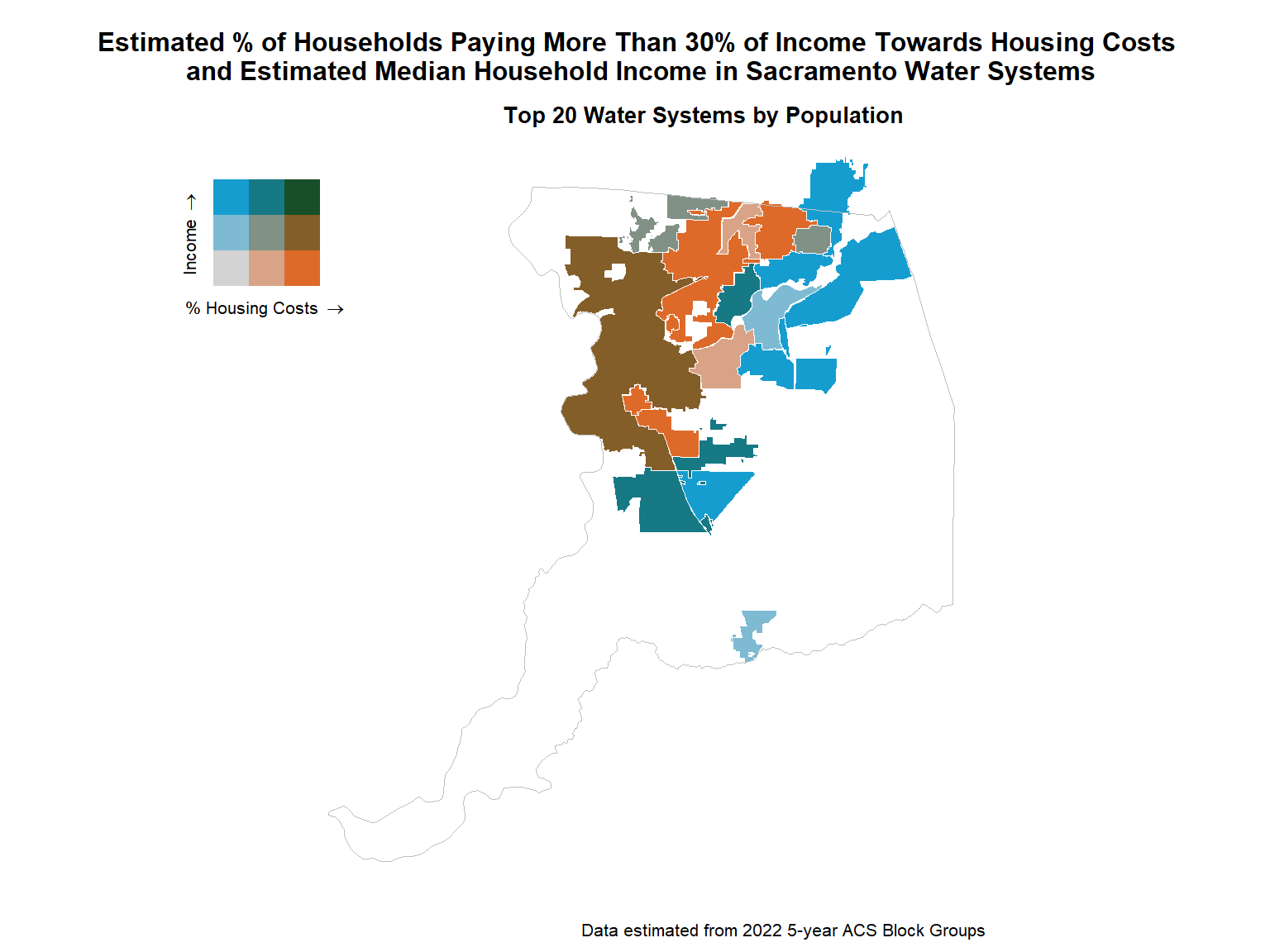
Figure 7 shows the same variables (relative housing costs and income) for the portions block groups overlapping Sacramento Suburban Water District – this illustrates the data underlying the interpolation process.
Code
# set defaults
biscale_pal_system <- 'BlueOr' # 'GrPink' # 'DkViolet2'
biscale_dim_system <- 3
# create classes
biscale_data_system <- bi_class(census_data_interpolate %>%
filter(water_system_name == system_plot) %>%
filter(!is.na(median_household_income)),
x = households_all_housing_costs_over30pct_percent,
y = median_household_income,
style = "quantile",
dim = biscale_dim_system)
# create map
biscale_map_system <- ggplot() +
geom_sf(data = biscale_data_system ,
mapping = aes(fill = bi_class),
color = "white",
size = 0.1,
show.legend = FALSE) +
bi_scale_fill(pal = biscale_pal_system,
dim = biscale_dim_system) +
labs(
title = glue("Estimated % of Households Paying More Than 30% of Income Towards Housing Costs \nand Estimated Median Household Income in {str_to_title(system_plot)}"),
# subtitle = glue(""),
caption = glue("Data from {acs_year} 5-year ACS Block Groups (Yellow = Missing Data)")#,
# title = glue("Housing Cost and Income \nin {str_to_title(system_plot)}"),
# caption = "% Housing cost shows the percent of households paying more than 30% of their income towards housing costs \nIncome shows median household income (yellow = missing)"#,
) +
# add the missing polygons back in
geom_sf(data = census_data_interpolate %>%
filter(water_system_name == system_plot) %>%
filter(is.na(median_household_income)),
color = "white",
fill = 'gold'
) +
bi_theme() +
theme(plot.title = element_text(size=12), # element_markdown(size=12)
plot.subtitle = element_text(size=10),
plot.caption = element_text(size=8, hjust = 1)) # element_markdown(size=8, hjust = 1))
# create legend
biscale_legend <- bi_legend(pal = biscale_pal_system,
dim = biscale_dim_system,
xlab = "% Housing Costs ",
ylab = "Income ",
size = 8)
# construct map
biscale_plot_system <- ggdraw() +
draw_plot(biscale_map_system, 0, 0, 1, 1) +
draw_plot(biscale_legend, 0.1, .55, 0.2, 0.2)
biscale_plot_system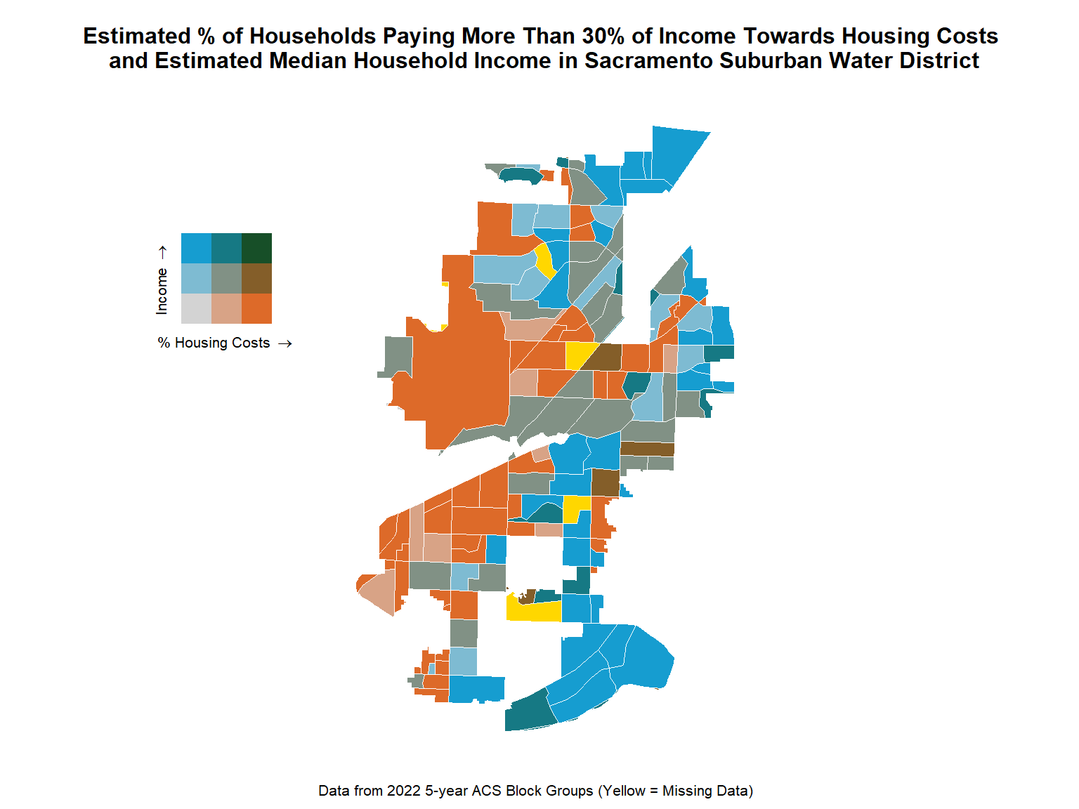
8 Check / Validate Results
We can apply a few additional checks to verify whether or not the calculations above are correct and/or whether the results are reasonable.
8.1 Check Count Variables Estimated with Areal Interpolation
As noted above, it’s possible to use pre-built functions for areal interpolation, and we can use those to double check the calculated count data above. For example, we can use the st_interpolate_aw function from the sf package (see Section 10 for use of a similar function from the areal R package):
# NOTE: it's only necessary to check the estimated values for one variable -
# this just checks the total estimated population
# interpolate with sf package
check_sf <- st_interpolate_aw(x = census_data_acs %>%
select(population_total_count),
to = water_systems_sac,
extensive = TRUE) %>%
bind_cols(water_systems_sac %>% st_drop_geometry)
# extract population estimates from sf package
pop_est_sf <- check_sf %>%
arrange(water_system_name) %>%
pull(population_total_count) %>%
round(0)
# extract population estimates from process above
pop_est_manual <- water_system_demographics %>%
arrange(water_system_name) %>%
pull(population_total_count) %>%
round(0)
# compare - should be TRUE if results are equivalent
all(pop_est_sf == pop_est_manual)[1] TRUE8.2 Compare Estimated vs Reported Population Estimates
[TO DO: Create map]
Based on the map above, it’s apparent that it’s likely difficult to obtain reasonable estimates for some suppliers, such as the suppliers with very small service areas in the southern portion of the county where the block groups are very large (and the supplier’s service are is only a small fraction of the total area of the block group). These issues are explored further in Section 11.
Note that there are a number of reasons why the estimated population values are likely to differ from the population numbers in the water system dataset (e.g., the depicted boundaries may not be correct or exact, the supplier may have used different methods to count/estimate the population they serve, the time frames for the estimates may be different, etc.). But, there may also be some cases where the numbers differ significantly – depending on the actual analysis being performed, this may mean that further work is needed for certain areas, or could mean that this method may not be sufficient and different methods are needed.
As a check, we can add a column to the interpolated dataset (which we’ll call population_percent_difference) to compute the difference between the estimated total population (in the population_total field) and the total population listed in the water_system_population_reported field (which is the reported value from the water system dataset).
water_system_demographics_check <- water_system_demographics %>%
left_join(water_systems_sac %>%
st_drop_geometry() %>%
select(water_system_name, water_system_population_reported,
water_system_service_connections),
by = 'water_system_name')
water_system_demographics_check <- water_system_demographics_check %>%
mutate(population_percent_difference =
round(100 * (population_total_count - water_system_population_reported) /
water_system_population_reported,
2),
.after = water_system_population_reported)For larger water systems, the estimated population values seem to be roughly in line with the population numbers in the original dataset– you can see this in the upper rows of Table 2.
Code
pct_format <- label_percent(accuracy = 0.01)
water_system_demographics_check %>%
st_drop_geometry() %>%
arrange(desc(water_system_population_reported)) %>%
select(water_system_name,
water_system_service_connections,
water_system_population_reported,
population_total_count,
population_percent_difference,
) %>%
mutate(population_percent_difference = pct_format(
population_percent_difference / 100)) %>%
rename('Water System Name' = water_system_name,
'Service Connections' = water_system_service_connections,
'Estimated Population' = population_total_count,
'Reported Population' = water_system_population_reported,
'Percent Difference' = population_percent_difference,
) %>%
kable(align = 'c',
format.args = list(big.mark = ',')
) %>%
scroll_box(height = "400px")| Water System Name | Service Connections | Reported Population | Estimated Population | Percent Difference |
|---|---|---|---|---|
| CITY OF SACRAMENTO MAIN | 142,794 | 510,931 | 516,189 | 1.03% |
| SACRAMENTO SUBURBAN WATER DISTRICT | 46,573 | 184,385 | 193,126 | 4.74% |
| SCWA - LAGUNA/VINEYARD | 47,411 | 172,666 | 145,495 | -15.74% |
| FOLSOM, CITY OF - MAIN | 21,424 | 68,122 | 62,462 | -8.31% |
| CITRUS HEIGHTS WATER DISTRICT | 19,940 | 65,911 | 68,912 | 4.55% |
| CALAM - SUBURBAN ROSEMONT | 16,238 | 53,563 | 57,897 | 8.09% |
| CALAM - PARKWAY | 14,779 | 48,738 | 58,635 | 20.31% |
| CALAM - LINCOLN OAKS | 14,390 | 47,487 | 42,916 | -9.63% |
| GOLDEN STATE WATER CO. - CORDOVA | 14,798 | 44,928 | 48,115 | 7.09% |
| ELK GROVE WATER SERVICE | 12,882 | 42,540 | 42,647 | 0.25% |
| CARMICHAEL WATER DISTRICT | 11,704 | 37,897 | 39,253 | 3.58% |
| FAIR OAKS WATER DISTRICT | 14,293 | 35,114 | 36,003 | 2.53% |
| CALAM - ANTELOPE | 10,528 | 34,720 | 33,120 | -4.61% |
| SAN JUAN WATER DISTRICT | 10,672 | 29,641 | 30,122 | 1.62% |
| GALT, CITY OF | 7,471 | 26,536 | 21,490 | -19.02% |
| SCWA MATHER-SUNRISE | 6,921 | 22,839 | 18,249 | -20.10% |
| ORANGE VALE WATER COMPANY | 5,684 | 18,005 | 17,387 | -3.43% |
| CAL AM FRUITRIDGE VISTA | 4,667 | 15,385 | 22,603 | 46.92% |
| RIO LINDA/ELVERTA COMMUNITY WATER DIST | 4,621 | 14,381 | 11,831 | -17.73% |
| SCWA - ARDEN PARK VISTA | 3,043 | 10,035 | 8,086 | -19.42% |
| FOLSOM STATE PRISON | 2,790 | 9,703 | 3,536 | -63.56% |
| FLORIN COUNTY WATER DISTRICT | 2,323 | 7,831 | 9,951 | 27.07% |
| RANCHO MURIETA COMMUNITY SERVI | 2,726 | 5,744 | 3,239 | -43.61% |
| GOLDEN STATE WATER CO - ARDEN WATER SERV | 1,716 | 5,125 | 6,556 | 27.92% |
| DEL PASO MANOR COUNTY WATER DI | 1,796 | 4,520 | 5,592 | 23.72% |
| CALAM - ARDEN | 1,185 | 3,908 | 10,112 | 158.75% |
| FOLSOM, CITY OF - ASHLAND | 1,079 | 3,538 | 3,845 | 8.68% |
| RIO COSUMNES CORRECTIONAL CENTER [SWS] | 13 | 2,800 | 22 | -99.21% |
| CALAM - ISLETON | 480 | 1,581 | 34 | -97.85% |
| MC CLELLAN MHP | 199 | 700 | 269 | -61.57% |
| CALAM - WALNUT GROVE | 197 | 651 | 12 | -98.16% |
| CALIFORNIA STATE FAIR | 269 | 650 | 532 | -18.15% |
| TOKAY PARK WATER CO | 198 | 525 | 652 | 24.19% |
| LAGUNA DEL SOL INC | 112 | 470 | 24 | -94.89% |
| OLYMPIA MOBILODGE | 200 | 450 | 290 | -35.56% |
| SAC CITY MOBILE HOME COMMUNITY LP | 164 | 350 | 229 | -34.57% |
| EAST WALNUT GROVE [SWS] | 166 | 300 | 3 | -99.00% |
| ELEVEN OAKS MOBILE HOME COMMUNITY | 136 | 262 | 233 | -11.07% |
| EL DORADO MOBILE HOME PARK | 128 | 256 | 139 | -45.70% |
| RANCHO MARINA | 77 | 250 | 0 | -100.00% |
| HOLIDAY MOBILE VILLAGE | 115 | 200 | 46 | -77.00% |
| IMPERIAL MANOR MOBILEHOME COMMUNITY | 186 | 200 | 209 | 4.50% |
| EL DORADO WEST MHP | 128 | 172 | 148 | -13.95% |
| KORTHS PIRATES LAIR | 64 | 150 | 0 | -100.00% |
| RIVER'S EDGE MARINA & RESORT | 83 | 150 | 0 | -100.00% |
| SOUTHWEST TRACT W M D [SWS] | 33 | 150 | 174 | 16.00% |
| VIEIRA'S RESORT, INC | 107 | 150 | 4 | -97.33% |
| B & W RESORT MARINA | 37 | 100 | 0 | -100.00% |
| HOOD WATER MAINTENCE DIST [SWS] | 82 | 100 | 1 | -99.00% |
| SPINDRIFT MARINA | 50 | 100 | 0 | -100.00% |
| LOCKE WATER WORKS CO [SWS] | 44 | 80 | 1 | -98.75% |
| WESTERNER MOBILE HOME PARK | 49 | 65 | 32 | -50.77% |
| HAPPY HARBOR (SWS) | 45 | 60 | 0 | -100.00% |
| SEQUOIA WATER ASSOC | 18 | 54 | 0 | -100.00% |
| PLANTATION MOBILE HOME PARK | 44 | 44 | 10 | -77.27% |
| TUNNEL TRAILER PARK | 21 | 44 | 0 | -100.00% |
| FREEPORT MARINA | 27 | 42 | 3 | -92.86% |
| EDGEWATER MOBILE HOME PARK | 22 | 40 | 0 | -100.00% |
| MAGNOLIA MUTUAL WATER | 34 | 40 | 1 | -97.50% |
| LINCOLN CHAN-HOME RANCH | 19 | 33 | 4 | -87.88% |
| LAGUNA VILLAGE RV PARK | 28 | 32 | 20 | -37.50% |
| DELTA CROSSING MHP | 22 | 30 | 0 | -100.00% |
But for water systems with a small population and/or service area, the estimated demographics may not match the reported population numbers from the water system dataset very well – you can see this in the top rows of Table 3. This probably indicates that, for small areas, some adjustments and/or further analysis may be needed, and the preliminary estimated values should be treated with some caution/skepticism.
Note: See Section 11 below for some more investigation into water systems whose estimated population is at or near zero.
Code
pct_format <- label_percent(accuracy = 0.01)
water_system_demographics_check %>%
st_drop_geometry() %>%
arrange(water_system_population_reported) %>%
select(water_system_name,
water_system_service_connections,
water_system_population_reported,
population_total_count,
population_percent_difference,
) %>%
mutate(population_percent_difference = pct_format(population_percent_difference / 100)) %>%
rename('Water System Name' = water_system_name,
'Service Connections' = water_system_service_connections,
'Estimated Population' = population_total_count,
'Reported Population' = water_system_population_reported,
'Percent Difference' = population_percent_difference,
) %>%
kable(align = 'c',
format.args = list(big.mark = ',')
) %>%
scroll_box(height = "400px")| Water System Name | Service Connections | Reported Population | Estimated Population | Percent Difference |
|---|---|---|---|---|
| DELTA CROSSING MHP | 22 | 30 | 0 | -100.00% |
| LAGUNA VILLAGE RV PARK | 28 | 32 | 20 | -37.50% |
| LINCOLN CHAN-HOME RANCH | 19 | 33 | 4 | -87.88% |
| EDGEWATER MOBILE HOME PARK | 22 | 40 | 0 | -100.00% |
| MAGNOLIA MUTUAL WATER | 34 | 40 | 1 | -97.50% |
| FREEPORT MARINA | 27 | 42 | 3 | -92.86% |
| PLANTATION MOBILE HOME PARK | 44 | 44 | 10 | -77.27% |
| TUNNEL TRAILER PARK | 21 | 44 | 0 | -100.00% |
| SEQUOIA WATER ASSOC | 18 | 54 | 0 | -100.00% |
| HAPPY HARBOR (SWS) | 45 | 60 | 0 | -100.00% |
| WESTERNER MOBILE HOME PARK | 49 | 65 | 32 | -50.77% |
| LOCKE WATER WORKS CO [SWS] | 44 | 80 | 1 | -98.75% |
| B & W RESORT MARINA | 37 | 100 | 0 | -100.00% |
| HOOD WATER MAINTENCE DIST [SWS] | 82 | 100 | 1 | -99.00% |
| SPINDRIFT MARINA | 50 | 100 | 0 | -100.00% |
| KORTHS PIRATES LAIR | 64 | 150 | 0 | -100.00% |
| RIVER'S EDGE MARINA & RESORT | 83 | 150 | 0 | -100.00% |
| SOUTHWEST TRACT W M D [SWS] | 33 | 150 | 174 | 16.00% |
| VIEIRA'S RESORT, INC | 107 | 150 | 4 | -97.33% |
| EL DORADO WEST MHP | 128 | 172 | 148 | -13.95% |
| HOLIDAY MOBILE VILLAGE | 115 | 200 | 46 | -77.00% |
| IMPERIAL MANOR MOBILEHOME COMMUNITY | 186 | 200 | 209 | 4.50% |
| RANCHO MARINA | 77 | 250 | 0 | -100.00% |
| EL DORADO MOBILE HOME PARK | 128 | 256 | 139 | -45.70% |
| ELEVEN OAKS MOBILE HOME COMMUNITY | 136 | 262 | 233 | -11.07% |
| EAST WALNUT GROVE [SWS] | 166 | 300 | 3 | -99.00% |
| SAC CITY MOBILE HOME COMMUNITY LP | 164 | 350 | 229 | -34.57% |
| OLYMPIA MOBILODGE | 200 | 450 | 290 | -35.56% |
| LAGUNA DEL SOL INC | 112 | 470 | 24 | -94.89% |
| TOKAY PARK WATER CO | 198 | 525 | 652 | 24.19% |
| CALIFORNIA STATE FAIR | 269 | 650 | 532 | -18.15% |
| CALAM - WALNUT GROVE | 197 | 651 | 12 | -98.16% |
| MC CLELLAN MHP | 199 | 700 | 269 | -61.57% |
| CALAM - ISLETON | 480 | 1,581 | 34 | -97.85% |
| RIO COSUMNES CORRECTIONAL CENTER [SWS] | 13 | 2,800 | 22 | -99.21% |
| FOLSOM, CITY OF - ASHLAND | 1,079 | 3,538 | 3,845 | 8.68% |
| CALAM - ARDEN | 1,185 | 3,908 | 10,112 | 158.75% |
| DEL PASO MANOR COUNTY WATER DI | 1,796 | 4,520 | 5,592 | 23.72% |
| GOLDEN STATE WATER CO - ARDEN WATER SERV | 1,716 | 5,125 | 6,556 | 27.92% |
| RANCHO MURIETA COMMUNITY SERVI | 2,726 | 5,744 | 3,239 | -43.61% |
| FLORIN COUNTY WATER DISTRICT | 2,323 | 7,831 | 9,951 | 27.07% |
| FOLSOM STATE PRISON | 2,790 | 9,703 | 3,536 | -63.56% |
| SCWA - ARDEN PARK VISTA | 3,043 | 10,035 | 8,086 | -19.42% |
| RIO LINDA/ELVERTA COMMUNITY WATER DIST | 4,621 | 14,381 | 11,831 | -17.73% |
| CAL AM FRUITRIDGE VISTA | 4,667 | 15,385 | 22,603 | 46.92% |
| ORANGE VALE WATER COMPANY | 5,684 | 18,005 | 17,387 | -3.43% |
| SCWA MATHER-SUNRISE | 6,921 | 22,839 | 18,249 | -20.10% |
| GALT, CITY OF | 7,471 | 26,536 | 21,490 | -19.02% |
| SAN JUAN WATER DISTRICT | 10,672 | 29,641 | 30,122 | 1.62% |
| CALAM - ANTELOPE | 10,528 | 34,720 | 33,120 | -4.61% |
| FAIR OAKS WATER DISTRICT | 14,293 | 35,114 | 36,003 | 2.53% |
| CARMICHAEL WATER DISTRICT | 11,704 | 37,897 | 39,253 | 3.58% |
| ELK GROVE WATER SERVICE | 12,882 | 42,540 | 42,647 | 0.25% |
| GOLDEN STATE WATER CO. - CORDOVA | 14,798 | 44,928 | 48,115 | 7.09% |
| CALAM - LINCOLN OAKS | 14,390 | 47,487 | 42,916 | -9.63% |
| CALAM - PARKWAY | 14,779 | 48,738 | 58,635 | 20.31% |
| CALAM - SUBURBAN ROSEMONT | 16,238 | 53,563 | 57,897 | 8.09% |
| CITRUS HEIGHTS WATER DISTRICT | 19,940 | 65,911 | 68,912 | 4.55% |
| FOLSOM, CITY OF - MAIN | 21,424 | 68,122 | 62,462 | -8.31% |
| SCWA - LAGUNA/VINEYARD | 47,411 | 172,666 | 145,495 | -15.74% |
| SACRAMENTO SUBURBAN WATER DISTRICT | 46,573 | 184,385 | 193,126 | 4.74% |
| CITY OF SACRAMENTO MAIN | 142,794 | 510,931 | 516,189 | 1.03% |
9 Alternative Computation Methods
As noted above in Section 6.1, in addition to the method described above, there are other methods that could be applied to estimate demographics of target areas (like water systems) from census data. Different methods may have their own strengths / weaknesses and applicable use cases. This section covers some other potential methods (but is not an exhaustive / comprehensive list of alternatives).
9.1 Simplified Method With MOE Estimates
Warning
This section is in progress.
As noted above, determining the margin of error (MOE) for estimates computed using areal weighted interpolation to aggregate portions of census units that overlap the target area of interest may not be possible (more research may be needed). If it’s necessary to compute MOEs for your aggregated values, and/or it’s preferable to use a simpler approach that doesn’t apply areal interpolation to assign fractional portions of census units to the target area, then a simplified method could be applied.
Tip
For guidance on how calculate MOEs for some types of derived estimates, see this document.
tidycensus has functions for calculating MOEs for derived estimates based on Census-supplied formulas, including moe_sum(), moe_product(), moe_ratio(), and moe_prop().
In this case, one option could be to use a minimum coverage threshold, where entire census units whose portion of area that overlaps the target area is greater than the threshold are treated as part of the target area, and any census units whose portion of area that overlaps the target area is less than the threshold are not treated as part of the target area (the threshold can be set to zero to use all census units that overlap the target area). But, when using a minimum coverage threshold, some water systems may not have any census units that meet the coverage threshold, so they may need to be accounted for separately (e.g., by selecting the overlapping census unit that has the greatest portion of overlap, as is done below), or those systems could be excluded from the calculation.
Warning
For small / medium sized target areas (small water systems), count data estimated using this method may be highly unreliable (since entire census units are used). In those cases, it’s likely that only the estimated rates / percentages may be useful, but it may be worth considering whether it’s worth making any estimates for those systems based on census data alone. See Section 9.1.2 and Section 11 for some further exploration of the issues when dealing with estimates for small areas from census data alone.
Because this approach operates on entire census units, the census bureau’s recommended approach for aggregating MOEs can be applied to produce an aggregated MOE. (However, keep in mind that the aggregated MOE applies to the uncertainty in the estimate for the census units included in the aggregation, and not may not necessarily capture the uncertainty in the estimate of the target area, since the two areas are now different – i.e., there is an additional un-quantified element of uncertainty/error which is not reflected in the MOE due to this mismatch. In general, any estimate which attempts to compute census demographics for areas that don’t align with the census boundaries may have some element of un-quantifiable error – more research/input may be needed.)
9.1.1 Compute Demographic Estimates
Here’s an example calculation.
9.1.1.1 Filter Census Units
First, determine which census units to include in the calculations:
# define threshold value -
## set to zero to use all census units that overlap the target area, set higher
## to require a larger % of any given census unit to overlap the target area to
## be included in estimates (e.g. 0.5 requires at least 50% of a census unit to
## overlap a water system to be included in the calculation for that water system)
overlap_threshold <- 0.5
# get census data (with MOEs) ----
census_data_acs_moe <- get_acs(geography = 'block group',
state = 'CA',
county = counties_list,
filter_by = water_systems_filter,
year = acs_year,
survey = 'acs5',
variables = census_vars_acs,
output = 'wide', # can be 'wide' or 'tidy'
geometry = TRUE,
cache_table = TRUE) %>%
st_transform(crs_projected) # convert to common coordinate system
# compute area of overlap for each census unit / water system ----
census_unit_overlap_simplified <- census_data_acs_moe %>%
mutate(census_unit_area = st_area(.)) %>%
st_intersection(water_systems_sac %>%
select(water_system_name)) %>%
mutate(clipped_area = st_area(.)) %>%
mutate(overlap_portion = drop_units(clipped_area / census_unit_area)) %>%
mutate(geoid_system = paste(GEOID, water_system_name, sep = '|')) %>%
st_drop_geometry()
# determine which census units to include, based on threshold value ----
census_unit_overlap_simplified <- census_unit_overlap_simplified %>%
mutate(above_threshold = overlap_portion >= overlap_threshold)
# account for water systems with no census units that meet the threshold value ----
### NOTE: may want to exclude this part to avoid making estimates for very small
### systems, which are not likely to be very reliable
## get list of systems with at least 1 census unit above threshold ----
systems_with_units_above_threshold <- census_unit_overlap_simplified %>%
filter(above_threshold == TRUE) %>%
pull(water_system_name) %>%
unique()
## get list of systems with no census units above threshold ----
systems_no_units_above_threshold <- water_systems_sac %>%
filter(!water_system_name %in% systems_with_units_above_threshold) %>%
pull(water_system_name)
## select the 1 census unit per system with the greatest overlap ----
census_units_keep_systems_no_units_above_threshold <- census_unit_overlap_simplified %>%
filter(water_system_name %in% systems_no_units_above_threshold) %>%
group_by(water_system_name) %>%
slice_max(order_by = overlap_portion, n = 1) %>%
ungroup()
# filter census units based on threshold value ----
### NOTE: this accounts for water systems with no census units that meet the
### threshold value - to avoid making estimates for those systems, remove the
### 'geoid_system_keep_below_threshold' variable below
## determine which census units to keep (for each water system) ----
geoid_system_keep_above_threshold <- census_unit_overlap_simplified %>%
filter(above_threshold == TRUE) %>%
pull(geoid_system)
geoid_system_keep_below_threshold <- census_units_keep_systems_no_units_above_threshold %>%
pull(geoid_system)
## filter census units ----
census_data_acs_moe <- census_data_acs_moe %>%
st_join(water_systems_sac %>% select(water_system_name)) %>%
mutate(geoid_system = paste(GEOID, water_system_name, sep = '|')) %>%
filter(geoid_system %in% c(geoid_system_keep_above_threshold,
geoid_system_keep_below_threshold))9.1.1.2 Calculated Count-Weighted Values
Next, compute weighted values for remaining variables, using estimated count data from the previous step (population or households) as weighting factors (as described above in Section 6.5):
# aggregate ----
water_system_demographics_simplified_method <- census_data_acs_moe %>%
# compute values for weighted variables
mutate(
average_household_size_weighted = average_household_sizeE * households_countE,
median_household_income_weighted = median_household_incomeE * households_countE,
per_capita_income_weighted = per_capita_incomeE * population_total_countE
) 9.1.1.3 Aggregate by Water System
Next, aggregate the data for each water system (as described above in Section 6.6) – do this by summing all of the count-based variables, and calculating weighted averages for all remaining count-weighted variables.
# compute aggregated values
water_system_demographics_simplified_method <- water_system_demographics_simplified_method %>%
# compute denominators for weighted variables
mutate(
average_household_size_denominator = if_else(
is.na(average_household_sizeE),
0,
households_countE),
median_household_income_denominator = if_else(
is.na(median_household_incomeE),
0,
households_countE),
per_capita_income_denominator = if_else(
is.na(per_capita_incomeE),
0,
population_total_countE)
) %>%
group_by(water_system_name) %>%
summarize(
across(
.cols = ends_with('_countE'),
.fns = ~ sum(.x)
),
average_household_size_hh_weighted =
sum(average_household_size_weighted, na.rm = TRUE) /
sum(average_household_size_denominator),
median_household_income_hh_weighted =
sum(median_household_income_weighted, na.rm = TRUE) /
sum(median_household_income_denominator),
per_capita_income_pop_weighted =
sum(per_capita_income_weighted, na.rm = TRUE) /
sum(per_capita_income_denominator)
) %>%
ungroup() %>%
# round weighted values
mutate(
across(
.cols = ends_with('_weighted'),
.fns = ~ round(.x, 2)
))
# if population / household counts are zero, set population / household weighted means values to NA
water_system_demographics_simplified_method <- water_system_demographics_simplified_method %>%
mutate(
average_household_size_hh_weighted = case_when(
households_countE == 0 ~ NA,
.default = average_household_size_hh_weighted
),
median_household_income_hh_weighted = case_when(
households_countE == 0 ~ NA,
.default = median_household_income_hh_weighted
),
per_capita_income_pop_weighted = case_when(
population_total_countE == 0 ~ NA,
.default = per_capita_income_pop_weighted
)
)Since computing a weighted mean for the median household income may be somewhat inaccurate (as noted above in Caution 1), it may also be worth calculating a grouped median household income based on the income bracket data:
# TO DO: Compute grouped median incomesUsing the aggregated data, compute additional metrics for each system, like ethnic/racial group portions, poverty rates, income distributions, etc.
# !!!! NOTE: may need to revise this section to calculate MOEs correctly !!!!
# compute rates / percentages ----
## race / ethnicity ----
water_system_demographics_simplified_method <- water_system_demographics_simplified_method %>%
mutate(
across(
.cols = starts_with('population_'),
.fns = ~ round(.x / population_total_countE * 100, 2),
.names = "{str_replace(.col, '_countE', '_percentE')}"
),
.after = population_multiple_countE) %>%
select(-population_total_percentE) # this always equals 1, not needed
## poverty rate ----
water_system_demographics_simplified_method <- water_system_demographics_simplified_method %>%
mutate(poverty_rate_percentE = case_when(
poverty_total_assessed_countE == 0 ~ 0,
.default = 100 * poverty_below_level_countE / poverty_total_assessed_countE
),
.after = poverty_above_level_countE)
# consistent income brackets ----
## 25k brackets ----
water_system_demographics_simplified_method <- water_system_demographics_simplified_method %>%
mutate(households_income_25k_brackets_0_25k_countE =
households_income_below_10k_countE +
households_income_10k_15k_countE +
households_income_15k_20k_countE +
households_income_20k_25k_countE,
households_income_25k_brackets_25k_50k_countE =
households_income_25k_30k_countE +
households_income_30k_35k_countE +
households_income_35k_40k_countE +
households_income_40k_45k_countE +
households_income_45k_50k_countE,
households_income_25k_brackets_50k_75k_countE =
households_income_50k_60k_countE +
households_income_60k_75k_countE,
.after = households_income_above_200k_countE
) # note - above 75k is already in 25k increments
## 50k brackets ----
water_system_demographics_simplified_method <- water_system_demographics_simplified_method %>%
mutate(households_income_50k_brackets_0_50k_countE =
households_income_below_10k_countE +
households_income_10k_15k_countE +
households_income_15k_20k_countE +
households_income_20k_25k_countE +
households_income_25k_30k_countE +
households_income_30k_35k_countE +
households_income_35k_40k_countE +
households_income_40k_45k_countE +
households_income_45k_50k_countE,
households_income_50k_brackets_50k_100k_countE =
households_income_50k_60k_countE +
households_income_60k_75k_countE +
households_income_75k_100k_countE,
households_income_50k_brackets_100k_150k_countE =
households_income_100k_125k_countE +
households_income_125k_150k_countE,
.after = households_income_25k_brackets_50k_75k_countE
) # above 150k is already in 50k increments
## portion of households paying more than 30% / 50% of income on housing ----
water_system_demographics_simplified_method <- water_system_demographics_simplified_method %>%
mutate(households_all_housing_costs_over30pct_percentE =
100 * (households_mortgage_housing_costs_over30pct_countE +
households_no_mortgage_housing_costs_over30pct_countE +
households_rent_housing_costs_over30pct_countE) /
households_countE,
.after = households_rent_housing_costs_over50pct_countE) %>%
mutate(households_all_housing_costs_over50pct_percentE =
100 * (households_mortgage_housing_costs_over50pct_countE +
households_no_mortgage_housing_costs_over50pct_countE +
households_rent_housing_costs_over50pct_countE) /
households_countE,
.after = households_all_housing_costs_over30pct_percentE)
# round values
water_system_demographics_simplified_method <- water_system_demographics_simplified_method %>%
mutate(
across(
.cols = ends_with('_countE'),
.fns = ~ round(.x, 0)
)) %>%
mutate(
across(
.cols = ends_with('_percentE'),
.fns = ~ round(.x, 2)
))
## NOTE: may want to calculate other rates / percentages, depending on project needsFinally, we can compute MOEs for the derived (estimated) data:
# compute MOEs
# [TO DO - use tidycensus functions to calculate MOEs for derived estimates]
# !!!! NOTE: may need to combine this with the section above to calculate MOEs correctly !!!![TO DO: insert results / plots of derived MOEs]
9.1.1.4 View Results
Table 4 shows the estimated demographics for each water system using the simplified interpolation method:
Code
pct_format <- label_percent(accuracy = 0.01)
water_system_demographics_simplified_method %>%
st_drop_geometry() %>%
mutate(across(
.cols = ends_with('_percent'),
.fns = ~ pct_format(. / 100))
) %>%
rename_with(.cols = everything(),
.fn = ~ str_replace_all(., pattern = '_', replacement = ' ') %>%
str_to_title(.)) %>%
kable(align = 'c',
format.args = list(big.mark = ',')
) %>%
scroll_box(height = "400px")| Water System Name | Population Total Counte | Population Hispanic Or Latino Counte | Population White Counte | Population Black Or African American Counte | Population Native American Or Alaska Native Counte | Population Asian Counte | Population Pacific Islander Counte | Population Other Counte | Population Multiple Counte | Population Hispanic Or Latino Percente | Population White Percente | Population Black Or African American Percente | Population Native American Or Alaska Native Percente | Population Asian Percente | Population Pacific Islander Percente | Population Other Percente | Population Multiple Percente | Poverty Total Assessed Counte | Poverty Below Level Counte | Poverty Above Level Counte | Poverty Rate Percente | Households Counte | Households Income Below 10k Counte | Households Income 10k 15k Counte | Households Income 15k 20k Counte | Households Income 20k 25k Counte | Households Income 25k 30k Counte | Households Income 30k 35k Counte | Households Income 35k 40k Counte | Households Income 40k 45k Counte | Households Income 45k 50k Counte | Households Income 50k 60k Counte | Households Income 60k 75k Counte | Households Income 75k 100k Counte | Households Income 100k 125k Counte | Households Income 125k 150k Counte | Households Income 150k 200k Counte | Households Income Above 200k Counte | Households Income 25k Brackets 0 25k Counte | Households Income 25k Brackets 25k 50k Counte | Households Income 25k Brackets 50k 75k Counte | Households Income 50k Brackets 0 50k Counte | Households Income 50k Brackets 50k 100k Counte | Households Income 50k Brackets 100k 150k Counte | Households Mortgage Total Counte | Households Mortgage Housing Costs Over30pct Counte | Households Mortgage Housing Costs Over50pct Counte | Households No Mortgage Total Counte | Households No Mortgage Housing Costs Over30pct Counte | Households No Mortgage Housing Costs Over50pct Counte | Households Rent Total Counte | Households Rent Housing Costs Over30pct Counte | Households Rent Housing Costs Over50pct Counte | Households All Housing Costs Over30pct Percente | Households All Housing Costs Over50pct Percente | Average Household Size Hh Weighted | Median Household Income Hh Weighted | Per Capita Income Pop Weighted |
|---|---|---|---|---|---|---|---|---|---|---|---|---|---|---|---|---|---|---|---|---|---|---|---|---|---|---|---|---|---|---|---|---|---|---|---|---|---|---|---|---|---|---|---|---|---|---|---|---|---|---|---|---|---|---|---|---|---|---|
| B & W RESORT MARINA | 770 | 319 | 404 | 0 | 0 | 35 | 0 | 0 | 12 | 41.43 | 52.47 | 0.00 | 0.00 | 4.55 | 0.00 | 0.00 | 1.56 | 770 | 174 | 596 | 22.60 | 380 | 29 | 30 | 11 | 15 | 18 | 8 | 23 | 18 | 4 | 49 | 29 | 17 | 71 | 23 | 0 | 35 | 85 | 71 | 78 | 156 | 95 | 94 | 143 | 89 | 28 | 154 | 45 | 40 | 83 | 20 | 15 | 40.53 | 21.84 | 2.03 | 51,977.00 | 40,522.00 |
| CAL AM FRUITRIDGE VISTA | 21,725 | 10,307 | 3,296 | 3,091 | 121 | 3,588 | 341 | 86 | 895 | 47.44 | 15.17 | 14.23 | 0.56 | 16.52 | 1.57 | 0.40 | 4.12 | 21,678 | 5,505 | 16,173 | 25.39 | 6,648 | 307 | 341 | 439 | 225 | 317 | 339 | 363 | 354 | 597 | 621 | 897 | 788 | 426 | 236 | 265 | 133 | 1,312 | 1,970 | 1,518 | 3,282 | 2,306 | 662 | 1,531 | 690 | 301 | 1,130 | 81 | 44 | 3,987 | 2,035 | 961 | 42.21 | 19.65 | 3.25 | 51,998.83 | 20,502.62 |
| CALAM - ANTELOPE | 35,144 | 5,501 | 20,603 | 3,580 | 120 | 3,137 | 84 | 205 | 1,914 | 15.65 | 58.62 | 10.19 | 0.34 | 8.93 | 0.24 | 0.58 | 5.45 | 35,090 | 3,891 | 31,199 | 11.09 | 11,231 | 338 | 244 | 102 | 103 | 135 | 526 | 240 | 362 | 497 | 903 | 1,168 | 1,675 | 1,601 | 1,119 | 1,225 | 993 | 787 | 1,760 | 2,071 | 2,547 | 3,746 | 2,720 | 5,748 | 1,898 | 578 | 1,853 | 189 | 111 | 3,630 | 1,951 | 749 | 35.95 | 12.80 | 3.12 | 92,904.62 | 34,473.58 |
| CALAM - ARDEN | 11,751 | 4,170 | 2,612 | 2,221 | 43 | 1,350 | 95 | 135 | 1,125 | 35.49 | 22.23 | 18.90 | 0.37 | 11.49 | 0.81 | 1.15 | 9.57 | 11,627 | 3,686 | 7,941 | 31.70 | 4,534 | 208 | 427 | 288 | 218 | 339 | 239 | 180 | 282 | 190 | 499 | 484 | 604 | 261 | 173 | 74 | 68 | 1,141 | 1,230 | 983 | 2,371 | 1,587 | 434 | 304 | 105 | 67 | 157 | 5 | 0 | 4,073 | 2,511 | 1,370 | 57.81 | 31.69 | 2.57 | 47,996.21 | 22,894.54 |
| CALAM - ISLETON | 770 | 319 | 404 | 0 | 0 | 35 | 0 | 0 | 12 | 41.43 | 52.47 | 0.00 | 0.00 | 4.55 | 0.00 | 0.00 | 1.56 | 770 | 174 | 596 | 22.60 | 380 | 29 | 30 | 11 | 15 | 18 | 8 | 23 | 18 | 4 | 49 | 29 | 17 | 71 | 23 | 0 | 35 | 85 | 71 | 78 | 156 | 95 | 94 | 143 | 89 | 28 | 154 | 45 | 40 | 83 | 20 | 15 | 40.53 | 21.84 | 2.03 | 51,977.00 | 40,522.00 |
| CALAM - LINCOLN OAKS | 42,879 | 9,381 | 26,242 | 1,196 | 147 | 2,790 | 282 | 247 | 2,594 | 21.88 | 61.20 | 2.79 | 0.34 | 6.51 | 0.66 | 0.58 | 6.05 | 42,820 | 4,106 | 38,714 | 9.59 | 15,597 | 752 | 362 | 290 | 645 | 483 | 616 | 576 | 645 | 730 | 1,070 | 1,628 | 2,526 | 1,879 | 1,242 | 1,488 | 665 | 2,049 | 3,050 | 2,698 | 5,099 | 5,224 | 3,121 | 7,373 | 2,742 | 946 | 3,353 | 489 | 295 | 4,871 | 2,564 | 1,304 | 37.15 | 16.32 | 2.73 | 79,787.31 | 33,102.60 |
| CALAM - PARKWAY | 58,185 | 18,554 | 8,847 | 6,745 | 8 | 19,176 | 1,328 | 135 | 3,392 | 31.89 | 15.20 | 11.59 | 0.01 | 32.96 | 2.28 | 0.23 | 5.83 | 57,985 | 9,906 | 48,079 | 17.08 | 17,611 | 1,117 | 760 | 514 | 693 | 736 | 648 | 702 | 679 | 712 | 1,152 | 1,912 | 2,438 | 1,638 | 1,493 | 1,530 | 887 | 3,084 | 3,477 | 3,064 | 6,561 | 5,502 | 3,131 | 7,016 | 2,718 | 1,057 | 3,357 | 634 | 379 | 7,238 | 3,588 | 2,066 | 39.41 | 19.89 | 3.27 | 72,236.22 | 27,248.18 |
| CALAM - SUBURBAN ROSEMONT | 56,906 | 13,814 | 24,365 | 7,788 | 92 | 6,628 | 377 | 245 | 3,597 | 24.28 | 42.82 | 13.69 | 0.16 | 11.65 | 0.66 | 0.43 | 6.32 | 56,674 | 8,350 | 48,324 | 14.73 | 20,572 | 1,145 | 591 | 495 | 698 | 647 | 572 | 569 | 869 | 622 | 1,270 | 2,503 | 3,304 | 2,540 | 1,510 | 1,642 | 1,595 | 2,929 | 3,279 | 3,773 | 6,208 | 7,077 | 4,050 | 8,063 | 2,245 | 719 | 3,276 | 424 | 270 | 9,233 | 4,467 | 2,309 | 34.69 | 16.03 | 2.74 | 80,780.02 | 34,123.00 |
| CALAM - WALNUT GROVE | 1,130 | 504 | 518 | 0 | 0 | 67 | 0 | 0 | 41 | 44.60 | 45.84 | 0.00 | 0.00 | 5.93 | 0.00 | 0.00 | 3.63 | 1,130 | 178 | 952 | 15.75 | 437 | 28 | 11 | 16 | 0 | 25 | 11 | 0 | 28 | 27 | 11 | 168 | 0 | 3 | 18 | 17 | 74 | 55 | 91 | 179 | 146 | 179 | 21 | 150 | 0 | 0 | 60 | 28 | 28 | 227 | 79 | 36 | 24.49 | 14.65 | 2.49 | 68,248.00 | 38,950.00 |
| CALIFORNIA STATE FAIR | 1,594 | 234 | 785 | 273 | 0 | 145 | 0 | 0 | 157 | 14.68 | 49.25 | 17.13 | 0.00 | 9.10 | 0.00 | 0.00 | 9.85 | 1,575 | 455 | 1,120 | 28.89 | 855 | 194 | 39 | 25 | 16 | 28 | 41 | 6 | 0 | 70 | 86 | 90 | 104 | 62 | 33 | 51 | 10 | 274 | 145 | 176 | 419 | 280 | 95 | 0 | 0 | 0 | 0 | 0 | 0 | 855 | 531 | 286 | 62.11 | 33.45 | 1.82 | 52,886.00 | 33,141.00 |
| CARMICHAEL WATER DISTRICT | 38,891 | 6,189 | 25,092 | 2,068 | 69 | 3,285 | 288 | 7 | 1,893 | 15.91 | 64.52 | 5.32 | 0.18 | 8.45 | 0.74 | 0.02 | 4.87 | 38,325 | 4,904 | 33,421 | 12.80 | 15,783 | 535 | 532 | 525 | 477 | 367 | 590 | 518 | 645 | 550 | 969 | 1,532 | 1,766 | 1,733 | 1,222 | 1,692 | 2,130 | 2,069 | 2,670 | 2,501 | 4,739 | 4,267 | 2,955 | 5,339 | 1,456 | 712 | 3,230 | 356 | 156 | 7,214 | 3,866 | 1,950 | 35.98 | 17.85 | 2.40 | 98,258.48 | 47,272.08 |
| CITRUS HEIGHTS WATER DISTRICT | 65,981 | 11,998 | 46,441 | 1,978 | 166 | 2,524 | 46 | 69 | 2,759 | 18.18 | 70.39 | 3.00 | 0.25 | 3.83 | 0.07 | 0.10 | 4.18 | 65,649 | 6,709 | 58,940 | 10.22 | 24,655 | 963 | 580 | 430 | 732 | 634 | 850 | 807 | 676 | 1,117 | 1,818 | 2,999 | 3,787 | 2,604 | 2,292 | 2,420 | 1,946 | 2,705 | 4,084 | 4,817 | 6,789 | 8,604 | 4,896 | 9,729 | 3,368 | 1,309 | 4,105 | 522 | 264 | 10,821 | 5,664 | 2,621 | 38.75 | 17.01 | 2.64 | 82,777.80 | 37,334.82 |
| CITY OF SACRAMENTO MAIN | 514,441 | 151,253 | 160,191 | 61,077 | 1,227 | 97,270 | 9,169 | 3,096 | 31,158 | 29.40 | 31.14 | 11.87 | 0.24 | 18.91 | 1.78 | 0.60 | 6.06 | 507,041 | 76,216 | 430,825 | 15.03 | 193,689 | 9,607 | 9,427 | 6,174 | 6,451 | 5,834 | 6,213 | 6,226 | 6,139 | 6,537 | 13,339 | 17,341 | 27,087 | 20,454 | 14,954 | 17,455 | 20,451 | 31,659 | 30,949 | 30,680 | 62,608 | 57,767 | 35,408 | 67,341 | 21,828 | 8,307 | 29,932 | 3,518 | 1,802 | 96,416 | 47,408 | 24,590 | 37.56 | 17.91 | 2.60 | 84,666.70 | 39,144.67 |
| DEL PASO MANOR COUNTY WATER DI | 6,194 | 758 | 4,398 | 439 | 15 | 150 | 32 | 20 | 382 | 12.24 | 71.00 | 7.09 | 0.24 | 2.42 | 0.52 | 0.32 | 6.17 | 6,194 | 711 | 5,483 | 11.48 | 2,421 | 193 | 53 | 53 | 74 | 24 | 59 | 76 | 242 | 43 | 172 | 301 | 168 | 189 | 144 | 366 | 264 | 373 | 444 | 473 | 817 | 641 | 333 | 1,052 | 387 | 212 | 601 | 132 | 85 | 768 | 531 | 131 | 43.37 | 17.68 | 2.56 | 90,552.53 | 39,800.86 |
| DELTA CROSSING MHP | 620 | 429 | 178 | 0 | 0 | 0 | 0 | 0 | 13 | 69.19 | 28.71 | 0.00 | 0.00 | 0.00 | 0.00 | 0.00 | 2.10 | 620 | 108 | 512 | 17.42 | 219 | 30 | 0 | 0 | 0 | 0 | 0 | 37 | 20 | 10 | 25 | 27 | 35 | 28 | 0 | 0 | 7 | 30 | 67 | 52 | 97 | 87 | 28 | 29 | 29 | 0 | 88 | 30 | 30 | 102 | 41 | 26 | 45.66 | 25.57 | 2.55 | 56,250.00 | 23,510.00 |
| EAST WALNUT GROVE [SWS] | 1,130 | 504 | 518 | 0 | 0 | 67 | 0 | 0 | 41 | 44.60 | 45.84 | 0.00 | 0.00 | 5.93 | 0.00 | 0.00 | 3.63 | 1,130 | 178 | 952 | 15.75 | 437 | 28 | 11 | 16 | 0 | 25 | 11 | 0 | 28 | 27 | 11 | 168 | 0 | 3 | 18 | 17 | 74 | 55 | 91 | 179 | 146 | 179 | 21 | 150 | 0 | 0 | 60 | 28 | 28 | 227 | 79 | 36 | 24.49 | 14.65 | 2.49 | 68,248.00 | 38,950.00 |
| EDGEWATER MOBILE HOME PARK | 743 | 29 | 663 | 24 | 0 | 0 | 0 | 0 | 27 | 3.90 | 89.23 | 3.23 | 0.00 | 0.00 | 0.00 | 0.00 | 3.63 | 743 | 267 | 476 | 35.94 | 414 | 72 | 69 | 21 | 23 | 16 | 5 | 4 | 19 | 11 | 0 | 57 | 30 | 53 | 0 | 12 | 22 | 185 | 55 | 57 | 240 | 87 | 53 | 71 | 30 | 30 | 255 | 27 | 7 | 88 | 59 | 59 | 28.02 | 23.19 | 1.79 | 38,125.00 | 33,103.00 |
| EL DORADO MOBILE HOME PARK | 2,539 | 1,530 | 198 | 266 | 0 | 337 | 0 | 0 | 208 | 60.26 | 7.80 | 10.48 | 0.00 | 13.27 | 0.00 | 0.00 | 8.19 | 2,523 | 1,088 | 1,435 | 43.12 | 878 | 102 | 177 | 0 | 67 | 103 | 14 | 0 | 137 | 27 | 132 | 8 | 17 | 0 | 79 | 0 | 15 | 346 | 281 | 140 | 627 | 157 | 79 | 58 | 0 | 0 | 176 | 97 | 97 | 644 | 313 | 176 | 46.70 | 31.09 | 2.71 | 29,468.00 | 17,394.00 |
| EL DORADO WEST MHP | 2,539 | 1,530 | 198 | 266 | 0 | 337 | 0 | 0 | 208 | 60.26 | 7.80 | 10.48 | 0.00 | 13.27 | 0.00 | 0.00 | 8.19 | 2,523 | 1,088 | 1,435 | 43.12 | 878 | 102 | 177 | 0 | 67 | 103 | 14 | 0 | 137 | 27 | 132 | 8 | 17 | 0 | 79 | 0 | 15 | 346 | 281 | 140 | 627 | 157 | 79 | 58 | 0 | 0 | 176 | 97 | 97 | 644 | 313 | 176 | 46.70 | 31.09 | 2.71 | 29,468.00 | 17,394.00 |
| ELEVEN OAKS MOBILE HOME COMMUNITY | 2,911 | 561 | 1,170 | 699 | 0 | 463 | 0 | 0 | 18 | 19.27 | 40.19 | 24.01 | 0.00 | 15.91 | 0.00 | 0.00 | 0.62 | 2,911 | 1,091 | 1,820 | 37.48 | 888 | 84 | 21 | 37 | 73 | 123 | 21 | 17 | 15 | 34 | 14 | 167 | 213 | 37 | 0 | 32 | 0 | 215 | 210 | 181 | 425 | 394 | 37 | 101 | 41 | 17 | 265 | 9 | 9 | 522 | 366 | 288 | 46.85 | 35.36 | 3.28 | 60,521.00 | 18,213.00 |
| ELK GROVE WATER SERVICE | 41,473 | 7,466 | 18,980 | 3,212 | 70 | 8,612 | 394 | 234 | 2,505 | 18.00 | 45.76 | 7.74 | 0.17 | 20.77 | 0.95 | 0.56 | 6.04 | 41,083 | 3,271 | 37,812 | 7.96 | 12,886 | 446 | 176 | 254 | 231 | 306 | 99 | 338 | 281 | 247 | 651 | 1,104 | 1,405 | 1,400 | 1,336 | 1,827 | 2,785 | 1,107 | 1,271 | 1,755 | 2,378 | 3,160 | 2,736 | 7,302 | 1,777 | 577 | 2,759 | 270 | 106 | 2,825 | 1,619 | 887 | 28.45 | 12.18 | 3.18 | 122,598.12 | 43,251.88 |
| FAIR OAKS WATER DISTRICT | 37,271 | 4,890 | 27,762 | 801 | 81 | 1,505 | 0 | 209 | 2,023 | 13.12 | 74.49 | 2.15 | 0.22 | 4.04 | 0.00 | 0.56 | 5.43 | 37,064 | 3,132 | 33,932 | 8.45 | 14,776 | 571 | 334 | 114 | 222 | 212 | 399 | 199 | 508 | 342 | 800 | 1,126 | 2,344 | 1,531 | 1,650 | 1,893 | 2,531 | 1,241 | 1,660 | 1,926 | 2,901 | 4,270 | 3,181 | 7,249 | 1,962 | 883 | 3,275 | 244 | 92 | 4,252 | 1,963 | 839 | 28.21 | 12.28 | 2.47 | 106,597.29 | 54,163.68 |
| FLORIN COUNTY WATER DISTRICT | 9,549 | 2,722 | 1,755 | 1,327 | 13 | 2,488 | 809 | 93 | 342 | 28.51 | 18.38 | 13.90 | 0.14 | 26.06 | 8.47 | 0.97 | 3.58 | 9,440 | 1,216 | 8,224 | 12.88 | 2,775 | 98 | 126 | 53 | 186 | 121 | 38 | 84 | 206 | 234 | 242 | 216 | 410 | 306 | 198 | 142 | 115 | 463 | 683 | 458 | 1,146 | 868 | 504 | 949 | 408 | 81 | 780 | 65 | 43 | 1,046 | 476 | 255 | 34.20 | 13.66 | 3.40 | 62,590.16 | 24,205.26 |
| FOLSOM STATE PRISON | 4,478 | 1,595 | 818 | 1,765 | 72 | 88 | 43 | 23 | 74 | 35.62 | 18.27 | 39.41 | 1.61 | 1.97 | 0.96 | 0.51 | 1.65 | 24 | 0 | 24 | 0.00 | 24 | 0 | 0 | 0 | 0 | 0 | 0 | 0 | 0 | 0 | 0 | 0 | 0 | 5 | 5 | 14 | 0 | 0 | 0 | 0 | 0 | 0 | 10 | 0 | 0 | 0 | 0 | 0 | 0 | 24 | 0 | 0 | 0.00 | 0.00 | NaN | 157,857.00 | 2,098.00 |
| FOLSOM, CITY OF - ASHLAND | 2,548 | 47 | 2,099 | 4 | 0 | 77 | 0 | 0 | 321 | 1.84 | 82.38 | 0.16 | 0.00 | 3.02 | 0.00 | 0.00 | 12.60 | 2,548 | 72 | 2,476 | 2.83 | 1,427 | 42 | 17 | 123 | 42 | 32 | 206 | 117 | 69 | 36 | 20 | 127 | 162 | 91 | 51 | 64 | 228 | 224 | 460 | 147 | 684 | 309 | 142 | 355 | 109 | 79 | 814 | 395 | 95 | 258 | 154 | 59 | 46.11 | 16.33 | 1.78 | 58,801.77 | 58,387.83 |
| FOLSOM, CITY OF - MAIN | 62,429 | 8,528 | 34,986 | 1,705 | 104 | 13,002 | 176 | 234 | 3,694 | 13.66 | 56.04 | 2.73 | 0.17 | 20.83 | 0.28 | 0.37 | 5.92 | 62,152 | 3,415 | 58,737 | 5.49 | 22,371 | 795 | 215 | 389 | 448 | 425 | 286 | 320 | 356 | 449 | 663 | 1,166 | 2,233 | 2,381 | 1,758 | 4,030 | 6,457 | 1,847 | 1,836 | 1,829 | 3,683 | 4,062 | 4,139 | 11,537 | 2,732 | 1,170 | 3,563 | 234 | 143 | 7,271 | 2,937 | 1,261 | 26.39 | 11.51 | 2.78 | 142,852.94 | 58,722.84 |
| FREEPORT MARINA | 620 | 429 | 178 | 0 | 0 | 0 | 0 | 0 | 13 | 69.19 | 28.71 | 0.00 | 0.00 | 0.00 | 0.00 | 0.00 | 2.10 | 620 | 108 | 512 | 17.42 | 219 | 30 | 0 | 0 | 0 | 0 | 0 | 37 | 20 | 10 | 25 | 27 | 35 | 28 | 0 | 0 | 7 | 30 | 67 | 52 | 97 | 87 | 28 | 29 | 29 | 0 | 88 | 30 | 30 | 102 | 41 | 26 | 45.66 | 25.57 | 2.55 | 56,250.00 | 23,510.00 |
| GALT, CITY OF | 22,226 | 9,620 | 10,323 | 530 | 25 | 870 | 0 | 0 | 858 | 43.28 | 46.45 | 2.38 | 0.11 | 3.91 | 0.00 | 0.00 | 3.86 | 22,065 | 1,372 | 20,693 | 6.22 | 7,125 | 136 | 170 | 267 | 201 | 132 | 338 | 148 | 348 | 134 | 559 | 716 | 836 | 1,083 | 557 | 837 | 663 | 774 | 1,100 | 1,275 | 1,874 | 2,111 | 1,640 | 3,855 | 934 | 538 | 1,399 | 95 | 35 | 1,871 | 958 | 447 | 27.89 | 14.32 | 3.09 | 91,799.24 | 33,555.54 |
| GOLDEN STATE WATER CO - ARDEN WATER SERV | 6,516 | 1,704 | 2,865 | 320 | 0 | 876 | 10 | 86 | 655 | 26.15 | 43.97 | 4.91 | 0.00 | 13.44 | 0.15 | 1.32 | 10.05 | 6,414 | 1,618 | 4,796 | 25.23 | 2,157 | 18 | 82 | 19 | 140 | 52 | 172 | 34 | 179 | 36 | 137 | 350 | 317 | 131 | 171 | 140 | 179 | 259 | 473 | 487 | 732 | 804 | 302 | 724 | 238 | 123 | 128 | 0 | 0 | 1,305 | 594 | 332 | 38.57 | 21.09 | 2.90 | 66,429.98 | 30,326.17 |
| GOLDEN STATE WATER CO. - CORDOVA | 50,516 | 9,770 | 27,252 | 4,121 | 229 | 6,223 | 183 | 221 | 2,517 | 19.34 | 53.95 | 8.16 | 0.45 | 12.32 | 0.36 | 0.44 | 4.98 | 50,236 | 4,624 | 45,612 | 9.20 | 18,844 | 508 | 492 | 346 | 493 | 519 | 472 | 414 | 471 | 621 | 1,342 | 1,768 | 2,737 | 2,677 | 1,780 | 2,022 | 2,182 | 1,839 | 2,497 | 3,110 | 4,336 | 5,847 | 4,457 | 7,842 | 2,278 | 873 | 3,630 | 368 | 198 | 7,372 | 2,810 | 1,483 | 28.95 | 13.55 | 2.66 | 97,368.09 | 42,709.89 |
| HAPPY HARBOR (SWS) | 743 | 29 | 663 | 24 | 0 | 0 | 0 | 0 | 27 | 3.90 | 89.23 | 3.23 | 0.00 | 0.00 | 0.00 | 0.00 | 3.63 | 743 | 267 | 476 | 35.94 | 414 | 72 | 69 | 21 | 23 | 16 | 5 | 4 | 19 | 11 | 0 | 57 | 30 | 53 | 0 | 12 | 22 | 185 | 55 | 57 | 240 | 87 | 53 | 71 | 30 | 30 | 255 | 27 | 7 | 88 | 59 | 59 | 28.02 | 23.19 | 1.79 | 38,125.00 | 33,103.00 |
| HOLIDAY MOBILE VILLAGE | 1,733 | 670 | 262 | 123 | 0 | 563 | 0 | 0 | 115 | 38.66 | 15.12 | 7.10 | 0.00 | 32.49 | 0.00 | 0.00 | 6.64 | 1,733 | 387 | 1,346 | 22.33 | 606 | 70 | 39 | 0 | 42 | 13 | 33 | 176 | 21 | 15 | 0 | 91 | 68 | 22 | 16 | 0 | 0 | 151 | 258 | 91 | 409 | 159 | 38 | 93 | 15 | 0 | 75 | 42 | 29 | 438 | 215 | 144 | 44.88 | 28.55 | 2.86 | 38,491.00 | 16,707.00 |
| HOOD WATER MAINTENCE DIST [SWS] | 620 | 429 | 178 | 0 | 0 | 0 | 0 | 0 | 13 | 69.19 | 28.71 | 0.00 | 0.00 | 0.00 | 0.00 | 0.00 | 2.10 | 620 | 108 | 512 | 17.42 | 219 | 30 | 0 | 0 | 0 | 0 | 0 | 37 | 20 | 10 | 25 | 27 | 35 | 28 | 0 | 0 | 7 | 30 | 67 | 52 | 97 | 87 | 28 | 29 | 29 | 0 | 88 | 30 | 30 | 102 | 41 | 26 | 45.66 | 25.57 | 2.55 | 56,250.00 | 23,510.00 |
| IMPERIAL MANOR MOBILEHOME COMMUNITY | 884 | 220 | 545 | 4 | 0 | 26 | 0 | 0 | 89 | 24.89 | 61.65 | 0.45 | 0.00 | 2.94 | 0.00 | 0.00 | 10.07 | 884 | 189 | 695 | 21.38 | 525 | 18 | 110 | 74 | 12 | 0 | 66 | 31 | 19 | 26 | 4 | 16 | 122 | 0 | 0 | 0 | 27 | 214 | 142 | 20 | 356 | 142 | 0 | 38 | 0 | 0 | 376 | 156 | 144 | 111 | 111 | 92 | 50.86 | 44.95 | 1.68 | 31,837.00 | 32,922.00 |
| KORTHS PIRATES LAIR | 743 | 29 | 663 | 24 | 0 | 0 | 0 | 0 | 27 | 3.90 | 89.23 | 3.23 | 0.00 | 0.00 | 0.00 | 0.00 | 3.63 | 743 | 267 | 476 | 35.94 | 414 | 72 | 69 | 21 | 23 | 16 | 5 | 4 | 19 | 11 | 0 | 57 | 30 | 53 | 0 | 12 | 22 | 185 | 55 | 57 | 240 | 87 | 53 | 71 | 30 | 30 | 255 | 27 | 7 | 88 | 59 | 59 | 28.02 | 23.19 | 1.79 | 38,125.00 | 33,103.00 |
| LAGUNA DEL SOL INC | 891 | 192 | 670 | 0 | 6 | 13 | 0 | 0 | 10 | 21.55 | 75.20 | 0.00 | 0.67 | 1.46 | 0.00 | 0.00 | 1.12 | 891 | 57 | 834 | 6.40 | 338 | 6 | 33 | 34 | 16 | 15 | 0 | 10 | 0 | 0 | 0 | 0 | 75 | 15 | 15 | 28 | 91 | 89 | 25 | 0 | 114 | 75 | 30 | 183 | 64 | 64 | 95 | 0 | 0 | 60 | 15 | 15 | 23.37 | 23.37 | 2.64 | 95,227.00 | 50,793.00 |
| LAGUNA VILLAGE RV PARK | 2,995 | 383 | 254 | 218 | 0 | 1,576 | 251 | 0 | 313 | 12.79 | 8.48 | 7.28 | 0.00 | 52.62 | 8.38 | 0.00 | 10.45 | 2,995 | 353 | 2,642 | 11.79 | 987 | 97 | 0 | 14 | 31 | 29 | 17 | 0 | 40 | 43 | 16 | 104 | 203 | 53 | 119 | 126 | 95 | 142 | 129 | 120 | 271 | 323 | 172 | 418 | 188 | 71 | 156 | 24 | 1 | 413 | 109 | 49 | 32.52 | 12.26 | 3.03 | 84,332.00 | 32,668.00 |
| LINCOLN CHAN-HOME RANCH | 1,130 | 504 | 518 | 0 | 0 | 67 | 0 | 0 | 41 | 44.60 | 45.84 | 0.00 | 0.00 | 5.93 | 0.00 | 0.00 | 3.63 | 1,130 | 178 | 952 | 15.75 | 437 | 28 | 11 | 16 | 0 | 25 | 11 | 0 | 28 | 27 | 11 | 168 | 0 | 3 | 18 | 17 | 74 | 55 | 91 | 179 | 146 | 179 | 21 | 150 | 0 | 0 | 60 | 28 | 28 | 227 | 79 | 36 | 24.49 | 14.65 | 2.49 | 68,248.00 | 38,950.00 |
| LOCKE WATER WORKS CO [SWS] | 1,130 | 504 | 518 | 0 | 0 | 67 | 0 | 0 | 41 | 44.60 | 45.84 | 0.00 | 0.00 | 5.93 | 0.00 | 0.00 | 3.63 | 1,130 | 178 | 952 | 15.75 | 437 | 28 | 11 | 16 | 0 | 25 | 11 | 0 | 28 | 27 | 11 | 168 | 0 | 3 | 18 | 17 | 74 | 55 | 91 | 179 | 146 | 179 | 21 | 150 | 0 | 0 | 60 | 28 | 28 | 227 | 79 | 36 | 24.49 | 14.65 | 2.49 | 68,248.00 | 38,950.00 |
| MAGNOLIA MUTUAL WATER | 1,130 | 504 | 518 | 0 | 0 | 67 | 0 | 0 | 41 | 44.60 | 45.84 | 0.00 | 0.00 | 5.93 | 0.00 | 0.00 | 3.63 | 1,130 | 178 | 952 | 15.75 | 437 | 28 | 11 | 16 | 0 | 25 | 11 | 0 | 28 | 27 | 11 | 168 | 0 | 3 | 18 | 17 | 74 | 55 | 91 | 179 | 146 | 179 | 21 | 150 | 0 | 0 | 60 | 28 | 28 | 227 | 79 | 36 | 24.49 | 14.65 | 2.49 | 68,248.00 | 38,950.00 |
| MC CLELLAN MHP | 2,911 | 561 | 1,170 | 699 | 0 | 463 | 0 | 0 | 18 | 19.27 | 40.19 | 24.01 | 0.00 | 15.91 | 0.00 | 0.00 | 0.62 | 2,911 | 1,091 | 1,820 | 37.48 | 888 | 84 | 21 | 37 | 73 | 123 | 21 | 17 | 15 | 34 | 14 | 167 | 213 | 37 | 0 | 32 | 0 | 215 | 210 | 181 | 425 | 394 | 37 | 101 | 41 | 17 | 265 | 9 | 9 | 522 | 366 | 288 | 46.85 | 35.36 | 3.28 | 60,521.00 | 18,213.00 |
| OLYMPIA MOBILODGE | 1,302 | 314 | 365 | 82 | 0 | 455 | 72 | 0 | 14 | 24.12 | 28.03 | 6.30 | 0.00 | 34.95 | 5.53 | 0.00 | 1.08 | 1,302 | 305 | 997 | 23.43 | 514 | 50 | 1 | 29 | 45 | 40 | 15 | 59 | 0 | 0 | 45 | 84 | 34 | 12 | 53 | 23 | 24 | 125 | 114 | 129 | 239 | 163 | 65 | 138 | 97 | 44 | 228 | 55 | 45 | 148 | 40 | 33 | 37.35 | 23.74 | 2.51 | 53,786.00 | 29,451.00 |
| ORANGE VALE WATER COMPANY | 18,135 | 3,076 | 12,612 | 274 | 76 | 672 | 98 | 39 | 1,288 | 16.96 | 69.55 | 1.51 | 0.42 | 3.71 | 0.54 | 0.22 | 7.10 | 18,034 | 2,028 | 16,006 | 11.25 | 6,714 | 381 | 95 | 68 | 104 | 238 | 55 | 281 | 113 | 163 | 346 | 761 | 1,032 | 965 | 699 | 645 | 768 | 648 | 850 | 1,107 | 1,498 | 2,139 | 1,664 | 3,377 | 984 | 441 | 1,673 | 327 | 191 | 1,664 | 674 | 304 | 29.57 | 13.94 | 2.67 | 92,866.38 | 41,992.51 |
| PLANTATION MOBILE HOME PARK | 1,733 | 670 | 262 | 123 | 0 | 563 | 0 | 0 | 115 | 38.66 | 15.12 | 7.10 | 0.00 | 32.49 | 0.00 | 0.00 | 6.64 | 1,733 | 387 | 1,346 | 22.33 | 606 | 70 | 39 | 0 | 42 | 13 | 33 | 176 | 21 | 15 | 0 | 91 | 68 | 22 | 16 | 0 | 0 | 151 | 258 | 91 | 409 | 159 | 38 | 93 | 15 | 0 | 75 | 42 | 29 | 438 | 215 | 144 | 44.88 | 28.55 | 2.86 | 38,491.00 | 16,707.00 |
| RANCHO MARINA | 743 | 29 | 663 | 24 | 0 | 0 | 0 | 0 | 27 | 3.90 | 89.23 | 3.23 | 0.00 | 0.00 | 0.00 | 0.00 | 3.63 | 743 | 267 | 476 | 35.94 | 414 | 72 | 69 | 21 | 23 | 16 | 5 | 4 | 19 | 11 | 0 | 57 | 30 | 53 | 0 | 12 | 22 | 185 | 55 | 57 | 240 | 87 | 53 | 71 | 30 | 30 | 255 | 27 | 7 | 88 | 59 | 59 | 28.02 | 23.19 | 1.79 | 38,125.00 | 33,103.00 |
| RANCHO MURIETA COMMUNITY SERVI | 2,943 | 684 | 1,891 | 58 | 9 | 197 | 0 | 38 | 66 | 23.24 | 64.25 | 1.97 | 0.31 | 6.69 | 0.00 | 1.29 | 2.24 | 2,943 | 198 | 2,745 | 6.73 | 1,318 | 54 | 37 | 0 | 0 | 0 | 17 | 84 | 29 | 97 | 37 | 43 | 101 | 108 | 216 | 207 | 288 | 91 | 227 | 80 | 318 | 181 | 324 | 1,015 | 216 | 114 | 212 | 52 | 52 | 91 | 52 | 52 | 24.28 | 16.54 | 2.23 | 146,106.87 | 67,805.56 |
| RIO COSUMNES CORRECTIONAL CENTER [SWS] | 1,379 | 355 | 517 | 232 | 41 | 62 | 25 | 80 | 67 | 25.74 | 37.49 | 16.82 | 2.97 | 4.50 | 1.81 | 5.80 | 4.86 | 276 | 0 | 276 | 0.00 | 80 | 0 | 0 | 0 | 0 | 0 | 0 | 19 | 0 | 0 | 0 | 7 | 0 | 39 | 15 | 0 | 0 | 0 | 19 | 7 | 19 | 7 | 54 | 54 | 0 | 0 | 7 | 0 | 0 | 19 | 19 | 0 | 23.75 | 0.00 | 3.45 | 115,897.00 | 11,095.00 |
| RIO LINDA/ELVERTA COMMUNITY WATER DIST | 12,192 | 2,590 | 7,846 | 362 | 9 | 871 | 21 | 79 | 414 | 21.24 | 64.35 | 2.97 | 0.07 | 7.14 | 0.17 | 0.65 | 3.40 | 12,192 | 1,722 | 10,470 | 14.12 | 3,914 | 211 | 171 | 68 | 177 | 65 | 115 | 152 | 100 | 137 | 192 | 274 | 580 | 485 | 461 | 474 | 252 | 627 | 569 | 466 | 1,196 | 1,046 | 946 | 1,969 | 574 | 168 | 797 | 118 | 44 | 1,148 | 569 | 397 | 32.22 | 15.56 | 3.09 | 83,285.07 | 33,660.07 |
| RIVER'S EDGE MARINA & RESORT | 743 | 29 | 663 | 24 | 0 | 0 | 0 | 0 | 27 | 3.90 | 89.23 | 3.23 | 0.00 | 0.00 | 0.00 | 0.00 | 3.63 | 743 | 267 | 476 | 35.94 | 414 | 72 | 69 | 21 | 23 | 16 | 5 | 4 | 19 | 11 | 0 | 57 | 30 | 53 | 0 | 12 | 22 | 185 | 55 | 57 | 240 | 87 | 53 | 71 | 30 | 30 | 255 | 27 | 7 | 88 | 59 | 59 | 28.02 | 23.19 | 1.79 | 38,125.00 | 33,103.00 |
| SAC CITY MOBILE HOME COMMUNITY LP | 1,346 | 480 | 101 | 44 | 0 | 721 | 0 | 0 | 0 | 35.66 | 7.50 | 3.27 | 0.00 | 53.57 | 0.00 | 0.00 | 0.00 | 1,346 | 648 | 698 | 48.14 | 525 | 65 | 95 | 53 | 58 | 45 | 0 | 0 | 25 | 12 | 39 | 8 | 78 | 22 | 25 | 0 | 0 | 271 | 82 | 47 | 353 | 125 | 47 | 21 | 9 | 9 | 90 | 9 | 0 | 414 | 239 | 177 | 48.95 | 35.43 | 2.53 | 22,380.00 | 16,689.00 |
| SACRAMENTO SUBURBAN WATER DISTRICT | 194,249 | 42,630 | 98,765 | 17,930 | 863 | 20,917 | 589 | 858 | 11,697 | 21.95 | 50.84 | 9.23 | 0.44 | 10.77 | 0.30 | 0.44 | 6.02 | 192,018 | 33,878 | 158,140 | 17.64 | 73,026 | 3,857 | 2,907 | 3,166 | 2,864 | 3,286 | 3,070 | 3,370 | 2,911 | 2,350 | 5,545 | 6,753 | 10,246 | 6,419 | 4,320 | 5,621 | 6,341 | 12,794 | 14,987 | 12,298 | 27,781 | 22,544 | 10,739 | 23,416 | 7,027 | 2,817 | 12,088 | 2,097 | 1,150 | 37,522 | 21,121 | 10,355 | 41.42 | 19.61 | 2.63 | 74,261.37 | 35,625.55 |
| SAN JUAN WATER DISTRICT | 33,974 | 3,762 | 24,292 | 877 | 358 | 2,904 | 16 | 114 | 1,651 | 11.07 | 71.50 | 2.58 | 1.05 | 8.55 | 0.05 | 0.34 | 4.86 | 33,844 | 1,944 | 31,900 | 5.74 | 12,190 | 435 | 173 | 111 | 277 | 149 | 164 | 113 | 168 | 152 | 507 | 847 | 1,203 | 1,025 | 961 | 1,209 | 4,696 | 996 | 746 | 1,354 | 1,742 | 2,557 | 1,986 | 7,042 | 1,987 | 767 | 3,340 | 571 | 355 | 1,808 | 823 | 374 | 27.74 | 12.27 | 2.77 | 158,425.50 | 72,077.20 |
| SCWA - ARDEN PARK VISTA | 6,785 | 741 | 5,476 | 21 | 11 | 224 | 7 | 38 | 267 | 10.92 | 80.71 | 0.31 | 0.16 | 3.30 | 0.10 | 0.56 | 3.94 | 6,785 | 167 | 6,618 | 2.46 | 2,700 | 34 | 0 | 0 | 41 | 27 | 21 | 0 | 18 | 143 | 76 | 137 | 132 | 486 | 163 | 364 | 1,058 | 75 | 209 | 213 | 284 | 345 | 649 | 1,804 | 540 | 90 | 622 | 59 | 17 | 274 | 101 | 35 | 25.93 | 5.26 | 2.51 | 157,292.32 | 97,133.30 |
| SCWA - LAGUNA/VINEYARD | 144,615 | 27,638 | 37,486 | 16,721 | 246 | 50,168 | 2,369 | 511 | 9,476 | 19.11 | 25.92 | 11.56 | 0.17 | 34.69 | 1.64 | 0.35 | 6.55 | 144,375 | 14,745 | 129,630 | 10.21 | 44,886 | 1,727 | 746 | 702 | 860 | 880 | 1,341 | 881 | 734 | 733 | 2,355 | 3,164 | 5,995 | 5,376 | 5,206 | 6,452 | 7,734 | 4,035 | 4,569 | 5,519 | 8,604 | 11,514 | 10,582 | 24,202 | 7,017 | 2,856 | 7,812 | 857 | 488 | 12,872 | 6,493 | 3,461 | 32.01 | 15.16 | 3.21 | 113,303.64 | 41,108.15 |
| SCWA MATHER-SUNRISE | 17,931 | 2,625 | 8,107 | 1,481 | 21 | 4,350 | 169 | 59 | 1,119 | 14.64 | 45.21 | 8.26 | 0.12 | 24.26 | 0.94 | 0.33 | 6.24 | 17,893 | 1,028 | 16,865 | 5.75 | 5,405 | 236 | 34 | 97 | 57 | 65 | 34 | 6 | 21 | 37 | 183 | 321 | 511 | 647 | 742 | 979 | 1,435 | 424 | 163 | 504 | 587 | 1,015 | 1,389 | 3,676 | 856 | 261 | 846 | 62 | 43 | 883 | 311 | 160 | 22.74 | 8.58 | 3.30 | 147,954.90 | 47,223.50 |
| SEQUOIA WATER ASSOC | 1,130 | 504 | 518 | 0 | 0 | 67 | 0 | 0 | 41 | 44.60 | 45.84 | 0.00 | 0.00 | 5.93 | 0.00 | 0.00 | 3.63 | 1,130 | 178 | 952 | 15.75 | 437 | 28 | 11 | 16 | 0 | 25 | 11 | 0 | 28 | 27 | 11 | 168 | 0 | 3 | 18 | 17 | 74 | 55 | 91 | 179 | 146 | 179 | 21 | 150 | 0 | 0 | 60 | 28 | 28 | 227 | 79 | 36 | 24.49 | 14.65 | 2.49 | 68,248.00 | 38,950.00 |
| SOUTHWEST TRACT W M D [SWS] | 2,002 | 332 | 490 | 274 | 31 | 863 | 12 | 0 | 0 | 16.58 | 24.48 | 13.69 | 1.55 | 43.11 | 0.60 | 0.00 | 0.00 | 2,002 | 437 | 1,565 | 21.83 | 653 | 7 | 24 | 80 | 0 | 83 | 0 | 0 | 118 | 134 | 36 | 28 | 53 | 0 | 15 | 24 | 51 | 111 | 335 | 64 | 446 | 117 | 15 | 37 | 12 | 0 | 96 | 0 | 0 | 520 | 331 | 81 | 52.53 | 12.40 | 3.04 | 45,671.00 | 36,348.00 |
| SPINDRIFT MARINA | 743 | 29 | 663 | 24 | 0 | 0 | 0 | 0 | 27 | 3.90 | 89.23 | 3.23 | 0.00 | 0.00 | 0.00 | 0.00 | 3.63 | 743 | 267 | 476 | 35.94 | 414 | 72 | 69 | 21 | 23 | 16 | 5 | 4 | 19 | 11 | 0 | 57 | 30 | 53 | 0 | 12 | 22 | 185 | 55 | 57 | 240 | 87 | 53 | 71 | 30 | 30 | 255 | 27 | 7 | 88 | 59 | 59 | 28.02 | 23.19 | 1.79 | 38,125.00 | 33,103.00 |
| TOKAY PARK WATER CO | 1,676 | 539 | 375 | 116 | 0 | 565 | 0 | 0 | 81 | 32.16 | 22.37 | 6.92 | 0.00 | 33.71 | 0.00 | 0.00 | 4.83 | 1,676 | 312 | 1,364 | 18.62 | 474 | 7 | 6 | 8 | 61 | 0 | 0 | 40 | 18 | 33 | 57 | 74 | 86 | 44 | 7 | 33 | 0 | 82 | 91 | 131 | 173 | 217 | 51 | 225 | 100 | 16 | 132 | 0 | 0 | 117 | 94 | 30 | 40.93 | 9.70 | 3.54 | 61,750.00 | 19,812.00 |
| TUNNEL TRAILER PARK | 581 | 289 | 203 | 0 | 0 | 27 | 0 | 0 | 62 | 49.74 | 34.94 | 0.00 | 0.00 | 4.65 | 0.00 | 0.00 | 10.67 | 581 | 0 | 581 | 0.00 | 197 | 0 | 0 | 0 | 17 | 0 | 0 | 0 | 0 | 0 | 31 | 0 | 16 | 21 | 0 | 112 | 0 | 17 | 0 | 31 | 17 | 47 | 21 | 91 | 32 | 0 | 67 | 8 | 0 | 39 | 0 | 0 | 20.30 | 0.00 | 2.95 | 153,092.00 | 42,507.00 |
| VIEIRA'S RESORT, INC | 770 | 319 | 404 | 0 | 0 | 35 | 0 | 0 | 12 | 41.43 | 52.47 | 0.00 | 0.00 | 4.55 | 0.00 | 0.00 | 1.56 | 770 | 174 | 596 | 22.60 | 380 | 29 | 30 | 11 | 15 | 18 | 8 | 23 | 18 | 4 | 49 | 29 | 17 | 71 | 23 | 0 | 35 | 85 | 71 | 78 | 156 | 95 | 94 | 143 | 89 | 28 | 154 | 45 | 40 | 83 | 20 | 15 | 40.53 | 21.84 | 2.03 | 51,977.00 | 40,522.00 |
| WESTERNER MOBILE HOME PARK | 3,479 | 612 | 613 | 985 | 19 | 1,091 | 0 | 0 | 159 | 17.59 | 17.62 | 28.31 | 0.55 | 31.36 | 0.00 | 0.00 | 4.57 | 3,430 | 815 | 2,615 | 23.76 | 1,085 | 115 | 0 | 12 | 12 | 73 | 15 | 48 | 67 | 0 | 236 | 100 | 104 | 196 | 12 | 76 | 19 | 139 | 203 | 336 | 342 | 440 | 208 | 429 | 205 | 94 | 94 | 36 | 36 | 562 | 376 | 190 | 56.87 | 29.49 | 3.16 | 59,296.00 | 23,437.00 |
9.1.2 Investigate / Check Assumptions
Figure 8 shows the census units used in this simplified method to estimate demographics for Sacramento Suburban Water District.
Code
mapview(census_data_acs_moe %>%
filter(water_system_name == system_plot),
alpha.regions = 0.8,
col.regions = 'grey60',
color = 'cyan',
# lwd = 1.3,
label = 'NAME',
layer.name = 'ACS Data',
legend = FALSE) + # zcol = 'NAME'
mapview(water_systems_sac %>%
filter(water_system_name == system_plot),
alpha.regions = 0.3,
col.regions = 'darkblue',
color = 'black',
lwd = 1.3,
zcol = 'water_system_name',
# label = 'water_system_name',
layer.name = 'Water System Boundary',
legend = FALSE)While this approach may work well for relatively large water systems (where the size of the system is significantly greater than the census units used for the analysis), for smaller water systems this method might be somewhat more problematic, as shown in Figure 9.
Code
system_plot_small <- 'RIO LINDA/ELVERTA COMMUNITY WATER DIST'
mapview(census_data_acs_moe %>%
filter(water_system_name == system_plot_small),
alpha.regions = 0.8,
col.regions = 'grey60',
color = 'cyan',
# lwd = 1.3,
label = 'NAME',
layer.name = 'ACS Data',
legend = FALSE) + # zcol = 'NAME'
mapview(water_systems_sac %>%
filter(water_system_name == system_plot_small),
alpha.regions = 0.3,
col.regions = 'darkblue',
color = 'black',
lwd = 1.3,
zcol = 'water_system_name',
# label = 'water_system_name',
layer.name = 'Water System Boundary',
legend = FALSE)Figure 10 shows another example of a small system – in this case there are large block groups which the water system only overlaps a small portion of.
Code
system_plot_small_2 <- 'RANCHO MURIETA COMMUNITY SERVI'
mapview(census_data_acs %>%
st_filter(water_systems_sac %>%
filter(water_system_name == system_plot_small_2)) %>%
filter(!GEOID %in% (census_data_acs_moe %>%
filter(water_system_name == system_plot_small_2) %>%
pull(GEOID))),
alpha.regions = 0.3,
col.regions = 'grey80',
color = 'grey30',
# lwd = 1.3,
label = 'NAME',
layer.name = 'ACS Data - Not Used',
legend = FALSE) + # zcol = 'NAME'
mapview(census_data_acs_moe %>%
filter(water_system_name == system_plot_small_2),
alpha.regions = 0.8,
col.regions = 'grey60',
color = 'cyan',
# lwd = 1.3,
label = 'NAME',
layer.name = 'ACS Data - Used',
legend = FALSE) + # zcol = 'NAME'
mapview(water_systems_sac %>%
filter(water_system_name == system_plot_small_2),
alpha.regions = 0.3,
col.regions = 'darkblue',
color = 'black',
lwd = 1.3,
zcol = 'water_system_name',
# label = 'water_system_name',
layer.name = 'Water System Boundary',
legend = FALSE)9.2 Population Weighted Areal Interpolation
The tidycensus package has a function for performing population weighted areal interpolation, interpolate_pw. Note that this is somewhat different than the population weighted interpolation procedure applied above in Section 6.5 (which starts with areal interpolation to estimate count data). Instead the interpolate_pw function “takes into account the distribution of the population within a Census unit to intelligently transfer data between incongruent units” – in more detail (from here):
An alternative method, population-weighted areal interpolation, can represent an improvement. As opposed to using area-based weights, population-weighted techniques estimate the populations of the intersections between origin and destination from a third dataset, then use those values for interpolation weights.
This method is implemented in tidycensus with the
interpolate_pw()function. This function is specified in a similar way tost_interpolate_aw(), but also requires a third dataset to be used as weights, and optionally a weight column to determine the relative influence of each feature in the weights dataset.
According to the documentation for the interpolate_pw function, the approach it implements is based on Esri’s data apportionment algorithm – more information about that can be found here and here.
Warning
Margins of error (MOEs) for estimated values cannot be calculated directly using the interpolate_pw function (and may be difficult to calculate at all) – the interpolate_pw documentation states: Margins of error in the ACS will not be transferred correctly with this function, so please use with caution
One drawback of using this approach is that it may not work well in cases where the overall area covered by the target area is significantly smaller than the area covered by the source dataset – for example, small water systems are often not given an estimated value using this method and NAs are returned for many of those areas (even if NA values are removed from the source data first). More research / feedback may be needed on how applicable this approach may be for certain use cases. It may also be somewhat difficult to explain and intrepret the results.
9.2.1 Interpolate
For these computations, we can use the ACS data that was accessed above in Section 5.2 and transformed in Section 6.3, and the decennial census data that was accessed above in Section 5.3.
9.2.1.1 Extensive (Count) Variables
First interpolate data for the ‘extensive’ (count) variables, by computing weighted sums for those variables:
# population weighted variables ----
water_system_demographics_interpolate_pw_extensive_pop <- interpolate_pw(
from = census_data_acs %>%
filter(!is.na(population_total_count)) %>%
select(starts_with(c('population_', 'poverty_')) & ends_with('_count')),
to = water_systems_sac,
to_id = 'water_system_name',
extensive = TRUE, # use TRUE for count data - returns weighted sums
weights = census_data_decennial,
# weight_placement = 'surface',
weight_column = 'population_total_count') %>%
mutate(across(
.cols = ends_with('_count'),
.fns = ~ round(.x, 0)
)) %>%
arrange(water_system_name)
# household weighted variables ----
water_system_demographics_interpolate_pw_extensive_hh <- interpolate_pw(
from = census_data_acs %>%
filter(!is.na(population_total_count)) %>%
select(starts_with('households_') & ends_with('_count')),
to = water_systems_sac,
to_id = 'water_system_name',
extensive = TRUE, # use TRUE for count data - returns weighted sums
weights = census_data_decennial,
# weight_placement = 'surface',
weight_column = 'households_count') %>%
mutate(across(
.cols = ends_with('_count'),
.fns = ~ round(.x, 0)
)) %>%
arrange(water_system_name) %>%
st_drop_geometry() # only need to keep geometry for 1 group - joining them all below9.2.2 Interpolate Intensive Variables
Then interpolate data for the remaining ‘intensive’ variables, by computing weighted means for those variables:
# population weighted variables ----
water_system_demographics_interpolate_pw_intensive_pop <- interpolate_pw(
from = census_data_acs %>%
filter(!is.na(population_total_count)) %>%
select(per_capita_income),
to = water_systems_sac,
to_id = 'water_system_name',
extensive = FALSE, # use FALSE to get weighted means
weights = census_data_decennial,
# weight_placement = 'surface',
weight_column = 'population_total_count') %>%
mutate(per_capita_income = round(per_capita_income, 0)) %>%
arrange(water_system_name) %>%
st_drop_geometry() # only need to keep geometry for 1 group - joining them all below
# household weighted variables ----
water_system_demographics_interpolate_pw_intensive_hh <- interpolate_pw(
from = census_data_acs %>%
filter(!is.na(population_total_count)) %>%
select(average_household_size,
median_household_income),
to = water_systems_sac,
to_id = 'water_system_name',
extensive = FALSE, # use FALSE to get weighted means
weights = census_data_decennial,
# weight_placement = 'surface',
weight_column = 'households_count') %>%
mutate(average_household_size = round(average_household_size, 2),
median_household_income = round(median_household_income, 0)) %>%
arrange(water_system_name) %>%
st_drop_geometry() # only need to keep geometry for 1 group - joining them all below9.2.3 Join All Variables
Then join the datasets with the two types of variables:
water_system_demographics_interpolate_pw <-
water_system_demographics_interpolate_pw_extensive_pop %>%
left_join(water_system_demographics_interpolate_pw_extensive_hh,
by = 'water_system_name') %>%
left_join(water_system_demographics_interpolate_pw_intensive_pop,
by = 'water_system_name') %>%
left_join(water_system_demographics_interpolate_pw_intensive_hh,
by = 'water_system_name')9.2.4 Compute Additional Aggregated Data
Since computing a weighted mean for the median household income may be somewhat inaccurate (as noted above in Caution 1), it may also be worth calculating a grouped median household income based on the income bracket data:
# TO DO: Compute grouped median incomesUsing the aggregated data, we can also compute some additional metrics for each system, like ethnic/racial group portions, poverty rates, income distributions, etc.:
# race / ethnicity ----
water_system_demographics_interpolate_pw <- water_system_demographics_interpolate_pw %>%
mutate(
across(
.cols = starts_with('population_'),
.fns = ~ ifelse(population_total_count == 0,
NA,
round(.x / population_total_count * 100, 2)),
.names = "{str_replace(.col, '_count', '_percent')}"
),
.after = population_multiple_count) %>%
select(-population_total_percent) # this always equals 1, not needed
# poverty rate ----
water_system_demographics_interpolate_pw <- water_system_demographics_interpolate_pw %>%
mutate(poverty_rate_percent = case_when(
population_total_count == 0 ~ NA,
poverty_total_assessed_count == 0 ~ 0,
.default = 100 * poverty_below_level_count / poverty_total_assessed_count
),
.after = poverty_above_level_count)
# consistent income brackets ----
## 25k brackets ----
water_system_demographics_interpolate_pw <- water_system_demographics_interpolate_pw %>%
mutate(households_income_25k_brackets_0_25k_count =
households_income_below_10k_count +
households_income_10k_15k_count +
households_income_15k_20k_count +
households_income_20k_25k_count,
households_income_25k_brackets_25k_50k_count =
households_income_25k_30k_count +
households_income_30k_35k_count +
households_income_35k_40k_count +
households_income_40k_45k_count +
households_income_45k_50k_count,
households_income_25k_brackets_50k_75k_count =
households_income_50k_60k_count +
households_income_60k_75k_count,
.after = households_income_above_200k_count
) # note: above 75k is already in 25k increments
## 50k brackets ----
water_system_demographics_interpolate_pw <- water_system_demographics_interpolate_pw %>%
mutate(households_income_50k_brackets_0_50k_count =
households_income_below_10k_count +
households_income_10k_15k_count +
households_income_15k_20k_count +
households_income_20k_25k_count +
households_income_25k_30k_count +
households_income_30k_35k_count +
households_income_35k_40k_count +
households_income_40k_45k_count +
households_income_45k_50k_count,
households_income_50k_brackets_50k_100k_count =
households_income_50k_60k_count +
households_income_60k_75k_count +
households_income_75k_100k_count,
households_income_50k_brackets_100k_150k_count =
households_income_100k_125k_count +
households_income_125k_150k_count,
.after = households_income_25k_brackets_50k_75k_count
) # note: above 150k is already in 50k increments
# portion of households paying more than 30% / 50% of income on housing ----
water_system_demographics_interpolate_pw <- water_system_demographics_interpolate_pw %>%
mutate(households_all_housing_costs_over30pct_percent =
ifelse(households_count == 0,
NA,
100 * (households_mortgage_housing_costs_over30pct_count +
households_no_mortgage_housing_costs_over30pct_count +
households_rent_housing_costs_over30pct_count) /
households_count),
.after = households_rent_housing_costs_over50pct_count) %>%
mutate(households_all_housing_costs_over50pct_percent =
ifelse(households_count == 0,
NA,
100 * (households_mortgage_housing_costs_over50pct_count +
households_no_mortgage_housing_costs_over50pct_count +
households_rent_housing_costs_over50pct_count) /
households_count
),
.after = households_all_housing_costs_over30pct_percent)
# round values ----
water_system_demographics_interpolate_pw <- water_system_demographics_interpolate_pw %>%
mutate(
across(
.cols = ends_with('_count'),
.fns = ~ round(.x, 0)
)) %>%
mutate(
across(
.cols = ends_with('_percent'),
.fns = ~ round(.x, 2)
))9.2.5 View Results
Note that this process returns NAs for 17 water systems, which generally appear to be relatively smaller systems.
Table 5 shows a comparison of the water system populations estimated using interpolate_pw and the reported system populations.
Code
pct_format <- label_percent(accuracy = 0.01)
water_system_demographics_interpolate_pw %>%
select(water_system_name, population_total_count) %>%
st_drop_geometry() %>%
left_join(water_systems_sac %>%
st_drop_geometry() %>%
select(water_system_service_connections,
water_system_population_reported,
water_system_name),
by = 'water_system_name') %>%
arrange(desc(water_system_population_reported)) %>%
relocate(water_system_service_connections, water_system_population_reported,
.before = population_total_count) %>%
mutate(population_percent_difference =
round(100 * (population_total_count - water_system_population_reported) /
water_system_population_reported,
2),
.after = population_total_count) %>%
mutate(population_percent_difference = pct_format(
population_percent_difference / 100)
) %>%
rename('Service Connections' = water_system_service_connections,
'Reported Population' = water_system_population_reported,
'Estimated Population' = population_total_count,
'Percent Difference' = population_percent_difference) %>%
kable(align = 'c',
format.args = list(big.mark = ',')) %>%
scroll_box(height = "400px")| water_system_name | Service Connections | Reported Population | Estimated Population | Percent Difference |
|---|---|---|---|---|
| CITY OF SACRAMENTO MAIN | 142,794 | 510,931 | 525,914 | 2.93% |
| SACRAMENTO SUBURBAN WATER DISTRICT | 46,573 | 184,385 | 190,956 | 3.56% |
| SCWA - LAGUNA/VINEYARD | 47,411 | 172,666 | 157,847 | -8.58% |
| FOLSOM, CITY OF - MAIN | 21,424 | 68,122 | 65,206 | -4.28% |
| CITRUS HEIGHTS WATER DISTRICT | 19,940 | 65,911 | 69,931 | 6.10% |
| CALAM - SUBURBAN ROSEMONT | 16,238 | 53,563 | 60,288 | 12.56% |
| CALAM - PARKWAY | 14,779 | 48,738 | 57,391 | 17.75% |
| CALAM - LINCOLN OAKS | 14,390 | 47,487 | 44,168 | -6.99% |
| GOLDEN STATE WATER CO. - CORDOVA | 14,798 | 44,928 | 48,645 | 8.27% |
| ELK GROVE WATER SERVICE | 12,882 | 42,540 | 42,834 | 0.69% |
| CARMICHAEL WATER DISTRICT | 11,704 | 37,897 | 39,773 | 4.95% |
| FAIR OAKS WATER DISTRICT | 14,293 | 35,114 | 38,819 | 10.55% |
| CALAM - ANTELOPE | 10,528 | 34,720 | 36,641 | 5.53% |
| SAN JUAN WATER DISTRICT | 10,672 | 29,641 | 30,997 | 4.57% |
| GALT, CITY OF | 7,471 | 26,536 | 27,287 | 2.83% |
| SCWA MATHER-SUNRISE | 6,921 | 22,839 | 19,629 | -14.05% |
| ORANGE VALE WATER COMPANY | 5,684 | 18,005 | 17,910 | -0.53% |
| CAL AM FRUITRIDGE VISTA | 4,667 | 15,385 | 21,116 | 37.25% |
| RIO LINDA/ELVERTA COMMUNITY WATER DIST | 4,621 | 14,381 | 15,102 | 5.01% |
| SCWA - ARDEN PARK VISTA | 3,043 | 10,035 | 9,617 | -4.17% |
| FOLSOM STATE PRISON | 2,790 | 9,703 | 32 | -99.67% |
| FLORIN COUNTY WATER DISTRICT | 2,323 | 7,831 | 11,114 | 41.92% |
| RANCHO MURIETA COMMUNITY SERVI | 2,726 | 5,744 | 4,853 | -15.51% |
| GOLDEN STATE WATER CO - ARDEN WATER SERV | 1,716 | 5,125 | 6,516 | 27.14% |
| DEL PASO MANOR COUNTY WATER DI | 1,796 | 4,520 | 5,784 | 27.96% |
| CALAM - ARDEN | 1,185 | 3,908 | 11,512 | 194.58% |
| FOLSOM, CITY OF - ASHLAND | 1,079 | 3,538 | 3,719 | 5.12% |
| RIO COSUMNES CORRECTIONAL CENTER [SWS] | 13 | 2,800 | NA | NA |
| CALAM - ISLETON | 480 | 1,581 | 519 | -67.17% |
| MC CLELLAN MHP | 199 | 700 | 412 | -41.14% |
| CALAM - WALNUT GROVE | 197 | 651 | 388 | -40.40% |
| CALIFORNIA STATE FAIR | 269 | 650 | NA | NA |
| TOKAY PARK WATER CO | 198 | 525 | 530 | 0.95% |
| LAGUNA DEL SOL INC | 112 | 470 | NA | NA |
| OLYMPIA MOBILODGE | 200 | 450 | 176 | -60.89% |
| SAC CITY MOBILE HOME COMMUNITY LP | 164 | 350 | NA | NA |
| EAST WALNUT GROVE [SWS] | 166 | 300 | 347 | 15.67% |
| ELEVEN OAKS MOBILE HOME COMMUNITY | 136 | 262 | 368 | 40.46% |
| EL DORADO MOBILE HOME PARK | 128 | 256 | 1,031 | 302.73% |
| RANCHO MARINA | 77 | 250 | NA | NA |
| HOLIDAY MOBILE VILLAGE | 115 | 200 | NA | NA |
| IMPERIAL MANOR MOBILEHOME COMMUNITY | 186 | 200 | 242 | 21.00% |
| EL DORADO WEST MHP | 128 | 172 | 227 | 31.98% |
| KORTHS PIRATES LAIR | 64 | 150 | NA | NA |
| RIVER'S EDGE MARINA & RESORT | 83 | 150 | NA | NA |
| SOUTHWEST TRACT W M D [SWS] | 33 | 150 | 183 | 22.00% |
| VIEIRA'S RESORT, INC | 107 | 150 | 67 | -55.33% |
| B & W RESORT MARINA | 37 | 100 | NA | NA |
| HOOD WATER MAINTENCE DIST [SWS] | 82 | 100 | 74 | -26.00% |
| SPINDRIFT MARINA | 50 | 100 | 13 | -87.00% |
| LOCKE WATER WORKS CO [SWS] | 44 | 80 | 76 | -5.00% |
| WESTERNER MOBILE HOME PARK | 49 | 65 | 20 | -69.23% |
| HAPPY HARBOR (SWS) | 45 | 60 | NA | NA |
| SEQUOIA WATER ASSOC | 18 | 54 | NA | NA |
| PLANTATION MOBILE HOME PARK | 44 | 44 | NA | NA |
| TUNNEL TRAILER PARK | 21 | 44 | NA | NA |
| FREEPORT MARINA | 27 | 42 | 105 | 150.00% |
| EDGEWATER MOBILE HOME PARK | 22 | 40 | NA | NA |
| MAGNOLIA MUTUAL WATER | 34 | 40 | 96 | 140.00% |
| LINCOLN CHAN-HOME RANCH | 19 | 33 | NA | NA |
| LAGUNA VILLAGE RV PARK | 28 | 32 | NA | NA |
| DELTA CROSSING MHP | 22 | 30 | NA | NA |
Table 6 shows all demographic variables estimated using the population weighted areal interpolation approach with the tidycensus interpolate_pw function.
Code
pct_format <- label_percent(accuracy = 0.01)
water_system_demographics_interpolate_pw %>%
st_drop_geometry() %>%
mutate(across(
.cols = ends_with('_percent'),
.fns = ~ pct_format(. / 100))
) %>%
rename_with(.cols = everything(),
.fn = ~ str_replace_all(., pattern = '_', replacement = ' ') %>%
str_to_title(.)) %>%
kable(align = 'c',
format.args = list(big.mark = ',')
) %>%
scroll_box(height = "400px")| Water System Name | Population Total Count | Population Hispanic Or Latino Count | Population White Count | Population Black Or African American Count | Population Native American Or Alaska Native Count | Population Asian Count | Population Pacific Islander Count | Population Other Count | Population Multiple Count | Population Hispanic Or Latino Percent | Population White Percent | Population Black Or African American Percent | Population Native American Or Alaska Native Percent | Population Asian Percent | Population Pacific Islander Percent | Population Other Percent | Population Multiple Percent | Poverty Total Assessed Count | Poverty Below Level Count | Poverty Above Level Count | Poverty Rate Percent | Households Count | Households Income Below 10k Count | Households Income 10k 15k Count | Households Income 15k 20k Count | Households Income 20k 25k Count | Households Income 25k 30k Count | Households Income 30k 35k Count | Households Income 35k 40k Count | Households Income 40k 45k Count | Households Income 45k 50k Count | Households Income 50k 60k Count | Households Income 60k 75k Count | Households Income 75k 100k Count | Households Income 100k 125k Count | Households Income 125k 150k Count | Households Income 150k 200k Count | Households Income Above 200k Count | Households Income 25k Brackets 0 25k Count | Households Income 25k Brackets 25k 50k Count | Households Income 25k Brackets 50k 75k Count | Households Income 50k Brackets 0 50k Count | Households Income 50k Brackets 50k 100k Count | Households Income 50k Brackets 100k 150k Count | Households Mortgage Total Count | Households Mortgage Housing Costs Over30pct Count | Households Mortgage Housing Costs Over50pct Count | Households No Mortgage Total Count | Households No Mortgage Housing Costs Over30pct Count | Households No Mortgage Housing Costs Over50pct Count | Households Rent Total Count | Households Rent Housing Costs Over30pct Count | Households Rent Housing Costs Over50pct Count | Households All Housing Costs Over30pct Percent | Households All Housing Costs Over50pct Percent | Per Capita Income | Average Household Size | Median Household Income |
|---|---|---|---|---|---|---|---|---|---|---|---|---|---|---|---|---|---|---|---|---|---|---|---|---|---|---|---|---|---|---|---|---|---|---|---|---|---|---|---|---|---|---|---|---|---|---|---|---|---|---|---|---|---|---|---|---|---|---|
| B & W RESORT MARINA | NA | NA | NA | NA | NA | NA | NA | NA | NA | NA | NA | NA | NA | NA | NA | NA | NA | NA | NA | NA | NA | NA | NA | NA | NA | NA | NA | NA | NA | NA | NA | NA | NA | NA | NA | NA | NA | NA | NA | NA | NA | NA | NA | NA | NA | NA | NA | NA | NA | NA | NA | NA | NA | NA | NA | NA | NA | NA |
| CAL AM FRUITRIDGE VISTA | 21,116 | 9,912 | 3,307 | 2,694 | 115 | 3,906 | 239 | 86 | 855 | 46.94% | 15.66% | 12.76% | 0.54% | 18.50% | 1.13% | 0.41% | 4.05% | 21,071 | 5,950 | 15,121 | 28.24% | 6,345 | 345 | 306 | 508 | 226 | 356 | 295 | 332 | 318 | 514 | 631 | 836 | 695 | 404 | 208 | 239 | 133 | 1,385 | 1,815 | 1,467 | 3,200 | 2,162 | 612 | 1,497 | 711 | 342 | 1,038 | 88 | 58 | 3,810 | 2,001 | 968 | 44.13% | 21.56% | 20,451 | 3.25 | 52,550 |
| CALAM - ANTELOPE | 36,641 | 5,854 | 21,441 | 3,550 | 134 | 3,192 | 75 | 275 | 2,119 | 15.98% | 58.52% | 9.69% | 0.37% | 8.71% | 0.20% | 0.75% | 5.78% | 36,527 | 3,694 | 32,833 | 10.11% | 11,842 | 365 | 221 | 108 | 144 | 123 | 515 | 275 | 408 | 497 | 837 | 1,203 | 1,890 | 1,646 | 1,230 | 1,299 | 1,082 | 838 | 1,818 | 2,040 | 2,656 | 3,930 | 2,876 | 6,196 | 2,076 | 718 | 1,920 | 199 | 120 | 3,726 | 1,925 | 736 | 35.47% | 13.29% | 35,072 | 3.17 | 94,331 |
| CALAM - ARDEN | 11,512 | 3,792 | 2,741 | 2,296 | 113 | 1,267 | 65 | 98 | 1,142 | 32.94% | 23.81% | 19.94% | 0.98% | 11.01% | 0.56% | 0.85% | 9.92% | 11,424 | 3,594 | 7,830 | 31.46% | 4,409 | 212 | 310 | 270 | 189 | 425 | 208 | 158 | 268 | 249 | 511 | 465 | 595 | 265 | 160 | 66 | 59 | 981 | 1,308 | 976 | 2,289 | 1,571 | 425 | 277 | 92 | 54 | 145 | 10 | 5 | 3,987 | 2,496 | 1,393 | 58.92% | 32.93% | 23,210 | 2.62 | 49,757 |
| CALAM - ISLETON | 519 | 215 | 272 | 0 | 0 | 24 | 0 | 0 | 8 | 41.43% | 52.41% | 0.00% | 0.00% | 4.62% | 0.00% | 0.00% | 1.54% | 519 | 117 | 401 | 22.54% | 235 | 18 | 19 | 7 | 9 | 11 | 5 | 14 | 11 | 2 | 30 | 18 | 11 | 44 | 14 | 0 | 22 | 53 | 43 | 48 | 96 | 59 | 58 | 89 | 55 | 17 | 95 | 28 | 25 | 51 | 12 | 9 | 40.43% | 21.70% | 40,522 | 2.03 | 51,977 |
| CALAM - LINCOLN OAKS | 44,168 | 9,337 | 27,315 | 1,566 | 143 | 2,744 | 299 | 238 | 2,526 | 21.14% | 61.84% | 3.55% | 0.32% | 6.21% | 0.68% | 0.54% | 5.72% | 44,067 | 4,131 | 39,936 | 9.37% | 15,916 | 750 | 392 | 297 | 654 | 471 | 606 | 563 | 633 | 640 | 1,084 | 1,663 | 2,519 | 1,908 | 1,312 | 1,582 | 840 | 2,093 | 2,913 | 2,747 | 5,006 | 5,266 | 3,220 | 7,710 | 2,817 | 965 | 3,411 | 519 | 312 | 4,795 | 2,445 | 1,289 | 36.32% | 16.12% | 33,847 | 2.73 | 82,056 |
| CALAM - PARKWAY | 57,391 | 18,307 | 8,731 | 6,680 | 16 | 18,900 | 1,311 | 138 | 3,309 | 31.90% | 15.21% | 11.64% | 0.03% | 32.93% | 2.28% | 0.24% | 5.77% | 57,206 | 9,646 | 47,560 | 16.86% | 17,388 | 1,045 | 738 | 501 | 706 | 681 | 637 | 733 | 710 | 726 | 1,133 | 1,916 | 2,466 | 1,598 | 1,471 | 1,509 | 819 | 2,990 | 3,487 | 3,049 | 6,477 | 5,515 | 3,069 | 7,044 | 2,725 | 1,057 | 3,320 | 626 | 372 | 7,024 | 3,474 | 1,877 | 39.25% | 19.01% | 27,100 | 3.26 | 72,531 |
| CALAM - SUBURBAN ROSEMONT | 60,288 | 14,475 | 25,934 | 7,866 | 92 | 7,477 | 403 | 252 | 3,791 | 24.01% | 43.02% | 13.05% | 0.15% | 12.40% | 0.67% | 0.42% | 6.29% | 60,053 | 8,956 | 51,098 | 14.91% | 21,905 | 1,196 | 622 | 512 | 761 | 705 | 583 | 623 | 929 | 658 | 1,327 | 2,607 | 3,521 | 2,740 | 1,650 | 1,717 | 1,754 | 3,091 | 3,498 | 3,934 | 6,589 | 7,455 | 4,390 | 8,482 | 2,323 | 767 | 3,612 | 438 | 280 | 9,811 | 4,769 | 2,461 | 34.38% | 16.01% | 34,894 | 2.71 | 80,855 |
| CALAM - WALNUT GROVE | 388 | 173 | 178 | 0 | 0 | 23 | 0 | 0 | 14 | 44.59% | 45.88% | 0.00% | 0.00% | 5.93% | 0.00% | 0.00% | 3.61% | 388 | 61 | 327 | 15.72% | 131 | 8 | 3 | 5 | 0 | 8 | 3 | 0 | 8 | 8 | 3 | 50 | 0 | 1 | 5 | 5 | 22 | 16 | 27 | 53 | 43 | 53 | 6 | 45 | 0 | 0 | 18 | 8 | 8 | 68 | 24 | 11 | 24.43% | 14.50% | 38,950 | 2.49 | 68,248 |
| CALIFORNIA STATE FAIR | NA | NA | NA | NA | NA | NA | NA | NA | NA | NA | NA | NA | NA | NA | NA | NA | NA | NA | NA | NA | NA | NA | NA | NA | NA | NA | NA | NA | NA | NA | NA | NA | NA | NA | NA | NA | NA | NA | NA | NA | NA | NA | NA | NA | NA | NA | NA | NA | NA | NA | NA | NA | NA | NA | NA | NA | NA | NA |
| CARMICHAEL WATER DISTRICT | 39,773 | 6,291 | 25,197 | 2,330 | 69 | 3,381 | 303 | 34 | 2,169 | 15.82% | 63.35% | 5.86% | 0.17% | 8.50% | 0.76% | 0.09% | 5.45% | 39,215 | 5,156 | 34,059 | 13.15% | 16,170 | 593 | 553 | 524 | 483 | 404 | 640 | 537 | 695 | 563 | 1,024 | 1,585 | 1,797 | 1,734 | 1,195 | 1,695 | 2,149 | 2,153 | 2,839 | 2,609 | 4,992 | 4,406 | 2,929 | 5,274 | 1,382 | 658 | 3,148 | 368 | 185 | 7,748 | 4,228 | 2,169 | 36.97% | 18.63% | 47,034 | 2.42 | 96,132 |
| CITRUS HEIGHTS WATER DISTRICT | 69,931 | 12,382 | 48,970 | 2,121 | 169 | 2,937 | 63 | 109 | 3,179 | 17.71% | 70.03% | 3.03% | 0.24% | 4.20% | 0.09% | 0.16% | 4.55% | 69,598 | 7,030 | 62,568 | 10.10% | 26,144 | 1,039 | 558 | 451 | 776 | 682 | 903 | 854 | 747 | 1,170 | 1,891 | 3,108 | 4,009 | 2,816 | 2,364 | 2,623 | 2,151 | 2,824 | 4,356 | 4,999 | 7,180 | 9,008 | 5,180 | 10,519 | 3,616 | 1,407 | 4,397 | 542 | 280 | 11,228 | 5,891 | 2,656 | 38.44% | 16.61% | 37,917 | 2.63 | 82,781 |
| CITY OF SACRAMENTO MAIN | 525,914 | 153,814 | 161,552 | 63,193 | 1,260 | 101,462 | 9,247 | 3,111 | 32,276 | 29.25% | 30.72% | 12.02% | 0.24% | 19.29% | 1.76% | 0.59% | 6.14% | 518,519 | 77,904 | 440,616 | 15.02% | 196,941 | 9,545 | 9,421 | 6,228 | 6,550 | 5,804 | 6,297 | 6,329 | 6,159 | 6,776 | 13,337 | 17,446 | 27,363 | 20,880 | 15,500 | 18,088 | 21,218 | 31,744 | 31,365 | 30,783 | 63,109 | 58,146 | 36,380 | 69,380 | 22,304 | 8,410 | 30,441 | 3,513 | 1,821 | 97,119 | 47,626 | 24,694 | 37.29% | 17.73% | 39,584 | 2.63 | 85,906 |
| DEL PASO MANOR COUNTY WATER DI | 5,784 | 704 | 4,109 | 413 | 15 | 129 | 32 | 20 | 360 | 12.17% | 71.04% | 7.14% | 0.26% | 2.23% | 0.55% | 0.35% | 6.22% | 5,784 | 659 | 5,125 | 11.39% | 2,327 | 186 | 51 | 53 | 72 | 23 | 55 | 72 | 240 | 40 | 167 | 286 | 164 | 180 | 134 | 354 | 249 | 362 | 430 | 453 | 792 | 617 | 314 | 992 | 359 | 203 | 586 | 126 | 81 | 749 | 519 | 124 | 43.15% | 17.53% | 41,038 | 2.53 | 91,599 |
| DELTA CROSSING MHP | NA | NA | NA | NA | NA | NA | NA | NA | NA | NA | NA | NA | NA | NA | NA | NA | NA | NA | NA | NA | NA | NA | NA | NA | NA | NA | NA | NA | NA | NA | NA | NA | NA | NA | NA | NA | NA | NA | NA | NA | NA | NA | NA | NA | NA | NA | NA | NA | NA | NA | NA | NA | NA | NA | NA | NA | NA | NA |
| EAST WALNUT GROVE [SWS] | 347 | 155 | 159 | 0 | 0 | 21 | 0 | 0 | 13 | 44.67% | 45.82% | 0.00% | 0.00% | 6.05% | 0.00% | 0.00% | 3.75% | 347 | 55 | 292 | 15.85% | 109 | 7 | 3 | 4 | 0 | 6 | 3 | 0 | 7 | 7 | 3 | 42 | 0 | 1 | 4 | 4 | 18 | 14 | 23 | 45 | 37 | 45 | 5 | 37 | 0 | 0 | 15 | 7 | 7 | 56 | 20 | 9 | 24.77% | 14.68% | 38,950 | 2.49 | 68,248 |
| EDGEWATER MOBILE HOME PARK | NA | NA | NA | NA | NA | NA | NA | NA | NA | NA | NA | NA | NA | NA | NA | NA | NA | NA | NA | NA | NA | NA | NA | NA | NA | NA | NA | NA | NA | NA | NA | NA | NA | NA | NA | NA | NA | NA | NA | NA | NA | NA | NA | NA | NA | NA | NA | NA | NA | NA | NA | NA | NA | NA | NA | NA | NA | NA |
| EL DORADO MOBILE HOME PARK | 1,031 | 622 | 80 | 108 | 0 | 137 | 0 | 0 | 85 | 60.33% | 7.76% | 10.48% | 0.00% | 13.29% | 0.00% | 0.00% | 8.24% | 1,025 | 442 | 583 | 43.12% | 352 | 41 | 71 | 0 | 27 | 41 | 6 | 0 | 55 | 11 | 53 | 3 | 7 | 0 | 32 | 0 | 6 | 139 | 113 | 56 | 252 | 63 | 32 | 23 | 0 | 0 | 71 | 39 | 39 | 258 | 126 | 71 | 46.88% | 31.25% | 17,394 | 2.71 | 29,468 |
| EL DORADO WEST MHP | 227 | 137 | 18 | 24 | 0 | 30 | 0 | 0 | 19 | 60.35% | 7.93% | 10.57% | 0.00% | 13.22% | 0.00% | 0.00% | 8.37% | 226 | 97 | 128 | 42.92% | 70 | 8 | 14 | 0 | 5 | 8 | 1 | 0 | 11 | 2 | 10 | 1 | 1 | 0 | 6 | 0 | 1 | 27 | 22 | 11 | 49 | 12 | 6 | 5 | 0 | 0 | 14 | 8 | 8 | 51 | 25 | 14 | 47.14% | 31.43% | 17,394 | 2.71 | 29,468 |
| ELEVEN OAKS MOBILE HOME COMMUNITY | 368 | 71 | 148 | 88 | 0 | 59 | 0 | 0 | 2 | 19.29% | 40.22% | 23.91% | 0.00% | 16.03% | 0.00% | 0.00% | 0.54% | 368 | 138 | 230 | 37.50% | 102 | 10 | 2 | 4 | 8 | 14 | 2 | 2 | 2 | 4 | 2 | 19 | 24 | 4 | 0 | 4 | 0 | 24 | 24 | 21 | 48 | 45 | 4 | 12 | 5 | 2 | 30 | 1 | 1 | 60 | 42 | 33 | 47.06% | 35.29% | 18,213 | 3.28 | 60,521 |
| ELK GROVE WATER SERVICE | 42,834 | 7,858 | 19,728 | 3,260 | 68 | 8,795 | 376 | 277 | 2,471 | 18.35% | 46.06% | 7.61% | 0.16% | 20.53% | 0.88% | 0.65% | 5.77% | 42,447 | 3,224 | 39,223 | 7.60% | 13,356 | 414 | 227 | 241 | 221 | 347 | 101 | 359 | 294 | 244 | 672 | 1,115 | 1,428 | 1,535 | 1,435 | 1,883 | 2,841 | 1,103 | 1,345 | 1,787 | 2,448 | 3,215 | 2,970 | 7,698 | 1,954 | 662 | 2,849 | 287 | 113 | 2,810 | 1,573 | 845 | 28.56% | 12.13% | 43,902 | 3.15 | 123,635 |
| FAIR OAKS WATER DISTRICT | 38,819 | 5,121 | 29,158 | 712 | 107 | 1,549 | 8 | 193 | 1,971 | 13.19% | 75.11% | 1.83% | 0.28% | 3.99% | 0.02% | 0.50% | 5.08% | 38,557 | 3,025 | 35,532 | 7.85% | 15,250 | 582 | 354 | 117 | 244 | 208 | 390 | 207 | 479 | 312 | 840 | 1,175 | 2,324 | 1,566 | 1,658 | 2,032 | 2,763 | 1,297 | 1,596 | 2,015 | 2,893 | 4,339 | 3,224 | 7,542 | 1,957 | 856 | 3,304 | 279 | 117 | 4,403 | 1,960 | 823 | 27.51% | 11.78% | 56,497 | 2.48 | 109,567 |
| FLORIN COUNTY WATER DISTRICT | 11,114 | 3,375 | 1,972 | 1,382 | 13 | 2,980 | 892 | 93 | 406 | 30.37% | 17.74% | 12.43% | 0.12% | 26.81% | 8.03% | 0.84% | 3.65% | 10,999 | 1,410 | 9,588 | 12.82% | 3,273 | 118 | 158 | 82 | 187 | 123 | 56 | 109 | 236 | 243 | 291 | 269 | 514 | 330 | 226 | 173 | 155 | 545 | 767 | 560 | 1,312 | 1,074 | 556 | 1,090 | 449 | 93 | 991 | 91 | 50 | 1,192 | 523 | 262 | 32.48% | 12.37% | 24,859 | 3.38 | 63,411 |
| FOLSOM STATE PRISON | 32 | 11 | 6 | 12 | 1 | 1 | 0 | 0 | 1 | 34.38% | 18.75% | 37.50% | 3.12% | 3.12% | 0.00% | 0.00% | 3.12% | 0 | 0 | 0 | 0.00% | 16 | 0 | 0 | 0 | 0 | 0 | 0 | 0 | 0 | 0 | 0 | 0 | 0 | 3 | 3 | 10 | 0 | 0 | 0 | 0 | 0 | 0 | 6 | 0 | 0 | 0 | 0 | 0 | 0 | 16 | 0 | 0 | 0.00% | 0.00% | 2,098 | NaN | 157,857 |
| FOLSOM, CITY OF - ASHLAND | 3,719 | 232 | 2,923 | 18 | 0 | 131 | 0 | 7 | 409 | 6.24% | 78.60% | 0.48% | 0.00% | 3.52% | 0.00% | 0.19% | 11.00% | 3,719 | 137 | 3,582 | 3.68% | 1,863 | 52 | 18 | 127 | 47 | 39 | 218 | 123 | 75 | 50 | 40 | 169 | 245 | 130 | 83 | 111 | 336 | 244 | 505 | 209 | 749 | 454 | 213 | 559 | 162 | 93 | 915 | 407 | 98 | 390 | 216 | 83 | 42.14% | 14.71% | 57,551 | 1.96 | 70,863 |
| FOLSOM, CITY OF - MAIN | 65,206 | 8,631 | 37,030 | 1,705 | 104 | 13,578 | 176 | 270 | 3,711 | 13.24% | 56.79% | 2.61% | 0.16% | 20.82% | 0.27% | 0.41% | 5.69% | 64,934 | 3,578 | 61,356 | 5.51% | 23,500 | 840 | 223 | 401 | 512 | 421 | 294 | 361 | 399 | 471 | 708 | 1,226 | 2,374 | 2,473 | 1,852 | 4,344 | 6,603 | 1,976 | 1,946 | 1,934 | 3,922 | 4,308 | 4,325 | 11,994 | 2,824 | 1,233 | 3,763 | 246 | 150 | 7,742 | 3,183 | 1,436 | 26.61% | 12.00% | 59,240 | 2.75 | 141,418 |
| FREEPORT MARINA | 105 | 73 | 30 | 0 | 0 | 0 | 0 | 0 | 2 | 69.52% | 28.57% | 0.00% | 0.00% | 0.00% | 0.00% | 0.00% | 1.90% | 105 | 18 | 87 | 17.14% | 33 | 4 | 0 | 0 | 0 | 0 | 0 | 6 | 3 | 2 | 4 | 4 | 5 | 4 | 0 | 0 | 1 | 4 | 11 | 8 | 15 | 13 | 4 | 4 | 4 | 0 | 13 | 4 | 4 | 15 | 6 | 4 | 42.42% | 24.24% | 23,510 | 2.55 | 56,250 |
| GALT, CITY OF | 27,287 | 11,655 | 12,708 | 556 | 24 | 1,211 | 34 | 7 | 1,093 | 42.71% | 46.57% | 2.04% | 0.09% | 4.44% | 0.12% | 0.03% | 4.01% | 27,128 | 1,932 | 25,196 | 7.12% | 8,755 | 205 | 187 | 361 | 255 | 172 | 387 | 193 | 398 | 193 | 657 | 841 | 941 | 1,237 | 637 | 1,054 | 1,037 | 1,008 | 1,343 | 1,498 | 2,351 | 2,439 | 1,874 | 4,690 | 1,174 | 688 | 2,053 | 203 | 82 | 2,013 | 980 | 456 | 26.92% | 14.00% | 34,695 | 3.06 | 92,548 |
| GOLDEN STATE WATER CO - ARDEN WATER SERV | 6,516 | 1,704 | 2,865 | 320 | 0 | 876 | 10 | 86 | 655 | 26.15% | 43.97% | 4.91% | 0.00% | 13.44% | 0.15% | 1.32% | 10.05% | 6,414 | 1,618 | 4,796 | 25.23% | 2,157 | 18 | 82 | 19 | 140 | 52 | 172 | 34 | 179 | 36 | 137 | 350 | 317 | 131 | 171 | 140 | 179 | 259 | 473 | 487 | 732 | 804 | 302 | 724 | 238 | 123 | 128 | 0 | 0 | 1,305 | 594 | 332 | 38.57% | 21.09% | 29,802 | 2.89 | 66,434 |
| GOLDEN STATE WATER CO. - CORDOVA | 48,645 | 8,725 | 26,541 | 4,055 | 229 | 6,209 | 183 | 221 | 2,481 | 17.94% | 54.56% | 8.34% | 0.47% | 12.76% | 0.38% | 0.45% | 5.10% | 48,365 | 4,409 | 43,956 | 9.12% | 18,345 | 619 | 485 | 302 | 488 | 466 | 453 | 385 | 467 | 578 | 1,301 | 1,659 | 2,688 | 2,566 | 1,721 | 1,996 | 2,172 | 1,894 | 2,349 | 2,960 | 4,243 | 5,648 | 4,287 | 7,679 | 2,223 | 858 | 3,519 | 368 | 198 | 7,147 | 2,688 | 1,391 | 28.78% | 13.34% | 43,978 | 2.63 | 97,985 |
| HAPPY HARBOR (SWS) | NA | NA | NA | NA | NA | NA | NA | NA | NA | NA | NA | NA | NA | NA | NA | NA | NA | NA | NA | NA | NA | NA | NA | NA | NA | NA | NA | NA | NA | NA | NA | NA | NA | NA | NA | NA | NA | NA | NA | NA | NA | NA | NA | NA | NA | NA | NA | NA | NA | NA | NA | NA | NA | NA | NA | NA | NA | NA |
| HOLIDAY MOBILE VILLAGE | NA | NA | NA | NA | NA | NA | NA | NA | NA | NA | NA | NA | NA | NA | NA | NA | NA | NA | NA | NA | NA | NA | NA | NA | NA | NA | NA | NA | NA | NA | NA | NA | NA | NA | NA | NA | NA | NA | NA | NA | NA | NA | NA | NA | NA | NA | NA | NA | NA | NA | NA | NA | NA | NA | NA | NA | NA | NA |
| HOOD WATER MAINTENCE DIST [SWS] | 74 | 51 | 21 | 0 | 0 | 0 | 0 | 0 | 2 | 68.92% | 28.38% | 0.00% | 0.00% | 0.00% | 0.00% | 0.00% | 2.70% | 74 | 13 | 61 | 17.57% | 12 | 2 | 0 | 0 | 0 | 0 | 0 | 2 | 1 | 1 | 1 | 2 | 2 | 2 | 0 | 0 | 0 | 2 | 4 | 3 | 6 | 5 | 2 | 2 | 2 | 0 | 5 | 2 | 2 | 6 | 2 | 1 | 50.00% | 25.00% | 23,510 | 2.55 | 56,250 |
| IMPERIAL MANOR MOBILEHOME COMMUNITY | 242 | 60 | 149 | 1 | 0 | 7 | 0 | 0 | 24 | 24.79% | 61.57% | 0.41% | 0.00% | 2.89% | 0.00% | 0.00% | 9.92% | 242 | 52 | 190 | 21.49% | 187 | 6 | 39 | 26 | 4 | 0 | 24 | 11 | 7 | 9 | 1 | 6 | 44 | 0 | 0 | 0 | 10 | 75 | 51 | 7 | 126 | 51 | 0 | 14 | 0 | 0 | 134 | 56 | 51 | 40 | 40 | 33 | 51.34% | 44.92% | 32,922 | 1.68 | 31,837 |
| KORTHS PIRATES LAIR | NA | NA | NA | NA | NA | NA | NA | NA | NA | NA | NA | NA | NA | NA | NA | NA | NA | NA | NA | NA | NA | NA | NA | NA | NA | NA | NA | NA | NA | NA | NA | NA | NA | NA | NA | NA | NA | NA | NA | NA | NA | NA | NA | NA | NA | NA | NA | NA | NA | NA | NA | NA | NA | NA | NA | NA | NA | NA |
| LAGUNA DEL SOL INC | NA | NA | NA | NA | NA | NA | NA | NA | NA | NA | NA | NA | NA | NA | NA | NA | NA | NA | NA | NA | NA | NA | NA | NA | NA | NA | NA | NA | NA | NA | NA | NA | NA | NA | NA | NA | NA | NA | NA | NA | NA | NA | NA | NA | NA | NA | NA | NA | NA | NA | NA | NA | NA | NA | NA | NA | NA | NA |
| LAGUNA VILLAGE RV PARK | NA | NA | NA | NA | NA | NA | NA | NA | NA | NA | NA | NA | NA | NA | NA | NA | NA | NA | NA | NA | NA | NA | NA | NA | NA | NA | NA | NA | NA | NA | NA | NA | NA | NA | NA | NA | NA | NA | NA | NA | NA | NA | NA | NA | NA | NA | NA | NA | NA | NA | NA | NA | NA | NA | NA | NA | NA | NA |
| LINCOLN CHAN-HOME RANCH | NA | NA | NA | NA | NA | NA | NA | NA | NA | NA | NA | NA | NA | NA | NA | NA | NA | NA | NA | NA | NA | NA | NA | NA | NA | NA | NA | NA | NA | NA | NA | NA | NA | NA | NA | NA | NA | NA | NA | NA | NA | NA | NA | NA | NA | NA | NA | NA | NA | NA | NA | NA | NA | NA | NA | NA | NA | NA |
| LOCKE WATER WORKS CO [SWS] | 76 | 34 | 35 | 0 | 0 | 5 | 0 | 0 | 3 | 44.74% | 46.05% | 0.00% | 0.00% | 6.58% | 0.00% | 0.00% | 3.95% | 76 | 12 | 64 | 15.79% | 32 | 2 | 1 | 1 | 0 | 2 | 1 | 0 | 2 | 2 | 1 | 12 | 0 | 0 | 1 | 1 | 5 | 4 | 7 | 13 | 11 | 13 | 1 | 11 | 0 | 0 | 4 | 2 | 2 | 17 | 6 | 3 | 25.00% | 15.62% | 38,950 | 2.49 | 68,248 |
| MAGNOLIA MUTUAL WATER | 96 | 43 | 44 | 0 | 0 | 6 | 0 | 0 | 3 | 44.79% | 45.83% | 0.00% | 0.00% | 6.25% | 0.00% | 0.00% | 3.12% | 96 | 15 | 81 | 15.62% | 36 | 2 | 1 | 1 | 0 | 2 | 1 | 0 | 2 | 2 | 1 | 14 | 0 | 0 | 1 | 1 | 6 | 4 | 7 | 15 | 11 | 15 | 1 | 12 | 0 | 0 | 5 | 2 | 2 | 19 | 6 | 3 | 22.22% | 13.89% | 38,950 | 2.49 | 68,248 |
| MC CLELLAN MHP | 412 | 79 | 165 | 99 | 0 | 65 | 0 | 0 | 3 | 19.17% | 40.05% | 24.03% | 0.00% | 15.78% | 0.00% | 0.00% | 0.73% | 412 | 154 | 257 | 37.38% | 170 | 16 | 4 | 7 | 14 | 24 | 4 | 3 | 3 | 6 | 3 | 32 | 41 | 7 | 0 | 6 | 0 | 41 | 40 | 35 | 81 | 76 | 7 | 19 | 8 | 3 | 51 | 2 | 2 | 100 | 70 | 55 | 47.06% | 35.29% | 18,213 | 3.28 | 60,521 |
| OLYMPIA MOBILODGE | 176 | 42 | 49 | 11 | 0 | 61 | 10 | 0 | 2 | 23.86% | 27.84% | 6.25% | 0.00% | 34.66% | 5.68% | 0.00% | 1.14% | 176 | 41 | 135 | 23.30% | 67 | 7 | 0 | 4 | 6 | 5 | 2 | 8 | 0 | 0 | 6 | 11 | 4 | 2 | 7 | 3 | 3 | 17 | 15 | 17 | 32 | 21 | 9 | 18 | 13 | 6 | 30 | 7 | 6 | 19 | 5 | 4 | 37.31% | 23.88% | 29,451 | 2.51 | 53,786 |
| ORANGE VALE WATER COMPANY | 17,910 | 2,705 | 12,640 | 251 | 267 | 636 | 90 | 37 | 1,283 | 15.10% | 70.58% | 1.40% | 1.49% | 3.55% | 0.50% | 0.21% | 7.16% | 17,805 | 1,987 | 15,818 | 11.16% | 6,827 | 411 | 130 | 73 | 96 | 228 | 60 | 281 | 127 | 182 | 370 | 760 | 1,055 | 933 | 643 | 679 | 800 | 710 | 878 | 1,130 | 1,588 | 2,185 | 1,576 | 3,394 | 1,125 | 459 | 1,726 | 335 | 203 | 1,707 | 699 | 319 | 31.62% | 14.37% | 42,789 | 2.60 | 92,925 |
| PLANTATION MOBILE HOME PARK | NA | NA | NA | NA | NA | NA | NA | NA | NA | NA | NA | NA | NA | NA | NA | NA | NA | NA | NA | NA | NA | NA | NA | NA | NA | NA | NA | NA | NA | NA | NA | NA | NA | NA | NA | NA | NA | NA | NA | NA | NA | NA | NA | NA | NA | NA | NA | NA | NA | NA | NA | NA | NA | NA | NA | NA | NA | NA |
| RANCHO MARINA | NA | NA | NA | NA | NA | NA | NA | NA | NA | NA | NA | NA | NA | NA | NA | NA | NA | NA | NA | NA | NA | NA | NA | NA | NA | NA | NA | NA | NA | NA | NA | NA | NA | NA | NA | NA | NA | NA | NA | NA | NA | NA | NA | NA | NA | NA | NA | NA | NA | NA | NA | NA | NA | NA | NA | NA | NA | NA |
| RANCHO MURIETA COMMUNITY SERVI | 4,853 | 958 | 3,223 | 213 | 9 | 313 | 0 | 38 | 99 | 19.74% | 66.41% | 4.39% | 0.19% | 6.45% | 0.00% | 0.78% | 2.04% | 4,849 | 228 | 4,621 | 4.70% | 2,068 | 68 | 47 | 0 | 11 | 10 | 43 | 95 | 81 | 97 | 75 | 140 | 154 | 155 | 273 | 365 | 453 | 126 | 326 | 215 | 452 | 369 | 428 | 1,494 | 314 | 143 | 402 | 78 | 66 | 172 | 56 | 52 | 21.66% | 12.62% | 65,767 | 2.33 | 140,014 |
| RIO COSUMNES CORRECTIONAL CENTER [SWS] | NA | NA | NA | NA | NA | NA | NA | NA | NA | NA | NA | NA | NA | NA | NA | NA | NA | NA | NA | NA | NA | NA | NA | NA | NA | NA | NA | NA | NA | NA | NA | NA | NA | NA | NA | NA | NA | NA | NA | NA | NA | NA | NA | NA | NA | NA | NA | NA | NA | NA | NA | NA | NA | NA | NA | NA | NA | NA |
| RIO LINDA/ELVERTA COMMUNITY WATER DIST | 15,102 | 3,244 | 9,844 | 375 | 28 | 947 | 23 | 115 | 526 | 21.48% | 65.18% | 2.48% | 0.19% | 6.27% | 0.15% | 0.76% | 3.48% | 15,100 | 1,961 | 13,140 | 12.99% | 4,809 | 201 | 174 | 76 | 220 | 79 | 141 | 150 | 144 | 139 | 221 | 395 | 771 | 673 | 567 | 521 | 335 | 671 | 653 | 616 | 1,324 | 1,387 | 1,240 | 2,472 | 702 | 187 | 948 | 139 | 60 | 1,388 | 678 | 454 | 31.59% | 14.58% | 33,391 | 3.15 | 85,765 |
| RIVER'S EDGE MARINA & RESORT | NA | NA | NA | NA | NA | NA | NA | NA | NA | NA | NA | NA | NA | NA | NA | NA | NA | NA | NA | NA | NA | NA | NA | NA | NA | NA | NA | NA | NA | NA | NA | NA | NA | NA | NA | NA | NA | NA | NA | NA | NA | NA | NA | NA | NA | NA | NA | NA | NA | NA | NA | NA | NA | NA | NA | NA | NA | NA |
| SAC CITY MOBILE HOME COMMUNITY LP | NA | NA | NA | NA | NA | NA | NA | NA | NA | NA | NA | NA | NA | NA | NA | NA | NA | NA | NA | NA | NA | NA | NA | NA | NA | NA | NA | NA | NA | NA | NA | NA | NA | NA | NA | NA | NA | NA | NA | NA | NA | NA | NA | NA | NA | NA | NA | NA | NA | NA | NA | NA | NA | NA | NA | NA | NA | NA |
| SACRAMENTO SUBURBAN WATER DISTRICT | 190,956 | 43,111 | 96,802 | 17,104 | 825 | 20,383 | 609 | 783 | 11,339 | 22.58% | 50.69% | 8.96% | 0.43% | 10.67% | 0.32% | 0.41% | 5.94% | 188,869 | 33,475 | 155,393 | 17.72% | 71,567 | 3,755 | 2,966 | 3,110 | 2,823 | 3,191 | 3,080 | 3,394 | 2,846 | 2,364 | 5,448 | 6,730 | 9,863 | 6,355 | 4,238 | 5,372 | 6,031 | 12,654 | 14,875 | 12,178 | 27,529 | 22,041 | 10,593 | 23,016 | 7,005 | 2,781 | 11,940 | 2,072 | 1,152 | 36,611 | 20,907 | 10,147 | 41.90% | 19.67% | 35,938 | 2.64 | 73,783 |
| SAN JUAN WATER DISTRICT | 30,997 | 3,454 | 22,175 | 822 | 196 | 2,816 | 16 | 84 | 1,434 | 11.14% | 71.54% | 2.65% | 0.63% | 9.08% | 0.05% | 0.27% | 4.63% | 30,881 | 1,652 | 29,229 | 5.35% | 11,004 | 370 | 140 | 81 | 286 | 134 | 173 | 107 | 132 | 116 | 521 | 704 | 945 | 939 | 867 | 1,066 | 4,423 | 877 | 662 | 1,225 | 1,539 | 2,170 | 1,806 | 6,380 | 1,752 | 752 | 2,993 | 530 | 337 | 1,630 | 716 | 316 | 27.24% | 12.77% | 74,432 | 2.79 | 161,995 |
| SCWA - ARDEN PARK VISTA | 9,617 | 1,186 | 6,855 | 490 | 11 | 513 | 9 | 79 | 473 | 12.33% | 71.28% | 5.10% | 0.11% | 5.33% | 0.09% | 0.82% | 4.92% | 9,540 | 842 | 8,698 | 8.83% | 4,046 | 176 | 70 | 90 | 97 | 91 | 55 | 27 | 81 | 197 | 186 | 260 | 343 | 545 | 246 | 451 | 1,131 | 433 | 451 | 446 | 884 | 789 | 791 | 1,953 | 579 | 145 | 772 | 90 | 29 | 1,321 | 670 | 404 | 33.09% | 14.29% | 75,992 | 2.30 | 129,121 |
| SCWA - LAGUNA/VINEYARD | 157,847 | 30,096 | 41,752 | 17,906 | 259 | 54,638 | 2,388 | 576 | 10,232 | 19.07% | 26.45% | 11.34% | 0.16% | 34.61% | 1.51% | 0.36% | 6.48% | 157,490 | 15,715 | 141,775 | 9.98% | 48,578 | 1,771 | 677 | 800 | 903 | 868 | 1,411 | 886 | 888 | 843 | 2,494 | 3,417 | 6,491 | 5,659 | 5,523 | 7,222 | 8,725 | 4,151 | 4,896 | 5,911 | 9,047 | 12,402 | 11,182 | 26,732 | 7,791 | 3,144 | 8,566 | 909 | 503 | 13,280 | 6,640 | 3,508 | 31.58% | 14.73% | 41,666 | 3.23 | 115,613 |
| SCWA MATHER-SUNRISE | 19,629 | 3,004 | 8,619 | 1,822 | 29 | 4,669 | 169 | 66 | 1,252 | 15.30% | 43.91% | 9.28% | 0.15% | 23.79% | 0.86% | 0.34% | 6.38% | 19,591 | 1,039 | 18,553 | 5.30% | 5,838 | 242 | 34 | 97 | 60 | 65 | 34 | 6 | 21 | 37 | 183 | 321 | 550 | 668 | 787 | 1,090 | 1,643 | 433 | 163 | 504 | 596 | 1,054 | 1,455 | 4,005 | 954 | 264 | 951 | 62 | 43 | 882 | 311 | 160 | 22.73% | 8.00% | 48,626 | 3.35 | 152,188 |
| SEQUOIA WATER ASSOC | NA | NA | NA | NA | NA | NA | NA | NA | NA | NA | NA | NA | NA | NA | NA | NA | NA | NA | NA | NA | NA | NA | NA | NA | NA | NA | NA | NA | NA | NA | NA | NA | NA | NA | NA | NA | NA | NA | NA | NA | NA | NA | NA | NA | NA | NA | NA | NA | NA | NA | NA | NA | NA | NA | NA | NA | NA | NA |
| SOUTHWEST TRACT W M D [SWS] | 183 | 30 | 45 | 25 | 3 | 79 | 1 | 0 | 0 | 16.39% | 24.59% | 13.66% | 1.64% | 43.17% | 0.55% | 0.00% | 0.00% | 183 | 40 | 143 | 21.86% | 67 | 1 | 2 | 8 | 0 | 8 | 0 | 0 | 12 | 14 | 4 | 3 | 5 | 0 | 2 | 2 | 5 | 11 | 34 | 7 | 45 | 12 | 2 | 4 | 1 | 0 | 10 | 0 | 0 | 53 | 34 | 8 | 52.24% | 11.94% | 36,348 | 3.04 | 45,671 |
| SPINDRIFT MARINA | 13 | 1 | 11 | 0 | 0 | 0 | 0 | 0 | 0 | 7.69% | 84.62% | 0.00% | 0.00% | 0.00% | 0.00% | 0.00% | 0.00% | 13 | 5 | 8 | 38.46% | 5 | 1 | 1 | 0 | 0 | 0 | 0 | 0 | 0 | 0 | 0 | 1 | 0 | 1 | 0 | 0 | 0 | 2 | 0 | 1 | 2 | 1 | 1 | 1 | 0 | 0 | 3 | 0 | 0 | 1 | 1 | 1 | 20.00% | 20.00% | 33,103 | 1.79 | 38,125 |
| TOKAY PARK WATER CO | 530 | 172 | 113 | 33 | 0 | 188 | 0 | 0 | 24 | 32.45% | 21.32% | 6.23% | 0.00% | 35.47% | 0.00% | 0.00% | 4.53% | 530 | 95 | 435 | 17.92% | 134 | 2 | 2 | 2 | 17 | 0 | 0 | 10 | 8 | 9 | 15 | 21 | 26 | 12 | 3 | 9 | 0 | 23 | 27 | 36 | 50 | 62 | 15 | 63 | 29 | 7 | 36 | 0 | 0 | 36 | 26 | 9 | 41.04% | 11.94% | 19,666 | 3.64 | 62,206 |
| TUNNEL TRAILER PARK | NA | NA | NA | NA | NA | NA | NA | NA | NA | NA | NA | NA | NA | NA | NA | NA | NA | NA | NA | NA | NA | NA | NA | NA | NA | NA | NA | NA | NA | NA | NA | NA | NA | NA | NA | NA | NA | NA | NA | NA | NA | NA | NA | NA | NA | NA | NA | NA | NA | NA | NA | NA | NA | NA | NA | NA | NA | NA |
| VIEIRA'S RESORT, INC | 67 | 28 | 35 | 0 | 0 | 3 | 0 | 0 | 1 | 41.79% | 52.24% | 0.00% | 0.00% | 4.48% | 0.00% | 0.00% | 1.49% | 67 | 15 | 52 | 22.39% | 44 | 3 | 3 | 1 | 2 | 2 | 1 | 3 | 2 | 0 | 6 | 3 | 2 | 8 | 3 | 0 | 4 | 9 | 8 | 9 | 17 | 11 | 11 | 17 | 10 | 3 | 18 | 5 | 5 | 10 | 2 | 2 | 38.64% | 22.73% | 40,522 | 2.03 | 51,977 |
| WESTERNER MOBILE HOME PARK | 20 | 4 | 4 | 6 | 0 | 6 | 0 | 0 | 1 | 20.00% | 20.00% | 30.00% | 0.00% | 30.00% | 0.00% | 0.00% | 5.00% | 20 | 5 | 15 | 25.00% | 16 | 2 | 0 | 0 | 0 | 1 | 0 | 1 | 1 | 0 | 3 | 1 | 2 | 3 | 0 | 1 | 0 | 2 | 3 | 4 | 5 | 6 | 3 | 6 | 3 | 1 | 1 | 1 | 1 | 8 | 6 | 3 | 62.50% | 31.25% | 23,437 | 3.16 | 59,296 |
9.3 Modified Population / Household Weighted Areal Interpolation
Warning
This section is in progress.
This section describes a method which is somewhat similar to the approach used in Section 9.2 above, in that it tries to account for variability in the distribution of the population within census units (block groups) by using more granular data from another source (block level data from the decennial census).
This method uses block and block group data from the decennial census to estimate the distribution of populations and households within census block groups, then applies those distributions to the block group data from the current ACS. Using those estimated distributions of populations/households within block groups, it then uses areal interpolation to estimate the portion of each block group’s count data to apply to the target area (water system boundary). Finally, it uses that estimated count data to compute weighted averages for remaining variables (e.g., per capita income, average household size, etc).
[TO DO: add example calculation]
9.4 Method Comparison
Warning
This section is in progress.
[TO DO: compare results across methods for certain variables - population, households, income, etc]
10 Detailed Population Estimates with Decennial Data
If you’re primarily interested in estimates of population/household counts alone (possibly including population by race/ethnicity, age, gender, etc.) as opposed to more detailed socioeconomic data (like income or poverty rates), in some cases it may make sense to use the block-level population data from the decennial census rather than block group level population data from the ACS. This method likely represents the most precise estimate of population (or other count data) that we can make from census data alone (i.e., without looking at other sources such as aerial imagery or parcel data).
Note
As described elsewhere, it may also be possible to use the block-level decennial population data as a way to estimate the distribution of the population within Census units and apply that information to the ACS data - see Section 9.2 and Section 9.3 above for methods which do that).
Since the decennial census only occurs once every 10 years, those estimates won’t necessarily reflect recent population changes (and will get generally be less accurate as the time since the last decennial census increases; however, keep in mind that even the 5-year ACS is an average that encompasses previous years’ estimates, so it also reflects some element of ‘historical’ data – for example, the 2022 5-year ACS reflects an average of data from 2018-2022). To reflect more recent population changes, one option may be to apply population projections or trends from historical records to scale the values calculated with this method.
Also, these values could simply be used to check the populations estimated from the ACS using any of the methods described above, and could help to flag areas where those methods are insufficient and more close inspection is needed.
10.1 Estimate Populations with Areal Interpolation
As a simple way to compute these estimates, we can use the aw_interpolate function from the areal package. This is similar to the st_interpolate_aw function from the sf package (see Section 8.1 for an example) – either one works, but the aw_interpolate function provides some additional options and documentation (for example, see here or here).
Note
There are some settings that you may need to modify in the aw_interpolate function depending on the type of analysis you’re doing. In particular, for more information about the weight argument – which can be either sum or total – see this section of the documentation. For more information about extensive versus intensive interpolations, see this section of the documentation (as noted above, the approaches described above avoid using areal interpolation to calculate intensive variables when count data associated with those variables that can be used as weighting factors – e.g. populations, households, etc. – are known; some of those considerations are discussed here; more research / input may be needed on that issue).
For these computations, we can use the decennial census data that was accessed above in Section 5.3.
# define variables to interpolate
vars_interpolate_aw <- census_data_decennial %>%
st_drop_geometry() %>%
select(ends_with('_count')) %>%
names()
# interpolate
water_system_population_estimates_blocks <- water_systems_sac %>%
aw_interpolate(tid = water_system_name,
source = census_data_decennial,
sid = GEOID,
weight = 'total',
extensive = vars_interpolate_aw)Here’s a view of the structure of the data that’s returned:
glimpse(water_system_population_estimates_blocks)Rows: 62
Columns: 22
$ water_system_name <chr> "HOOD WATER MAINTENC…
$ water_system_number <chr> "CA3400101", "CA3400…
$ water_system_id <chr> "{36268DB3-9DB2-4305…
$ water_system_boundary_type <chr> "Water Service Area"…
$ water_system_owner_type <chr> "L", "P", "P", "P", …
$ water_system_county <chr> "SACRAMENTO", "SACRA…
$ water_system_regulating_agency <chr> "LPA64 - SACRAMENTO …
$ water_system_federal_class <chr> "COMMUNITY", "COMMUN…
$ water_system_state_class <chr> "COMMUNITY", "COMMUN…
$ water_system_service_connections <dbl> 82, 199, 34, 64, 128…
$ water_system_population_reported <dbl> 100, 700, 40, 150, 2…
$ households_count <dbl> 23.3434672, 163.6072…
$ population_asian_count <dbl> 2.151173620, 14.2501…
$ population_black_or_african_american_count <dbl> 0.00000000, 20.05259…
$ population_hispanic_or_latino_count <dbl> 31.78662034, 77.9684…
$ population_multiple_count <dbl> 1.14905862, 47.88558…
$ population_native_american_or_alaska_native_count <dbl> 8.298117231, 0.77231…
$ population_other_count <dbl> 0.60257947514, 3.119…
$ population_pacific_islander_count <dbl> 0.151173620, 6.35812…
$ population_total_count <dbl> 71.3434991, 376.0814…
$ population_white_count <dbl> 27.2047762, 205.6748…
$ geometry <GEOMETRY [m]> MULTIPOLYGO…We can also add fields with each racial/ethnic group’s estimated percent of the total population within each water system’s service area, and round all results:
water_system_population_estimates_blocks <- water_system_population_estimates_blocks %>%
mutate(
across(
.cols = starts_with('population_'),
.fns = ~ round(.x / population_total_count * 100, 2),
.names = "{str_replace(.col, '_count', '_percent')}"
),
.after = population_white_count) %>%
select(-population_total_percent) # this always equals 1, not needed
# clean
water_system_population_estimates_blocks <- water_system_population_estimates_blocks %>%
mutate(
across(
.cols = ends_with('_count'),
.fns = ~ round(.x, 0)
)
)
# select fields to keep
water_system_population_estimates_blocks <- water_system_population_estimates_blocks %>%
select(water_system_name, water_system_number,
water_system_service_connections, water_system_population_reported,
ends_with('_count'), ends_with('_percent')) %>%
relocate(population_total_count, .after = water_system_population_reported) %>%
relocate(households_count, .before = geometry) %>%
arrange(water_system_name)10.2 View Results
Table 7 shows a comparison of the system populations estimated using the block-level data from the 2020 Decennial Census and the reported system populations.
Code
pct_format <- label_percent(accuracy = 0.01)
water_system_population_estimates_blocks %>%
st_drop_geometry() %>%
select(water_system_name, water_system_service_connections,
water_system_population_reported, population_total_count) %>%
arrange(desc(water_system_population_reported)) %>%
mutate(population_percent_difference =
round(100 * (population_total_count - water_system_population_reported) /
water_system_population_reported,
2),
.after = population_total_count) %>%
mutate(population_percent_difference = pct_format(
population_percent_difference / 100)) %>%
rename('Service Connections' = water_system_service_connections,
'Reported Population' = water_system_population_reported,
'Estimated Population' = population_total_count,
'Percent Difference' = population_percent_difference) %>%
kable(align = 'c',
format.args = list(big.mark = ',')) %>%
scroll_box(height = "400px")| water_system_name | Service Connections | Reported Population | Estimated Population | Percent Difference |
|---|---|---|---|---|
| CITY OF SACRAMENTO MAIN | 142,794 | 510,931 | 526,939 | 3.13% |
| SACRAMENTO SUBURBAN WATER DISTRICT | 46,573 | 184,385 | 193,282 | 4.83% |
| SCWA - LAGUNA/VINEYARD | 47,411 | 172,666 | 159,610 | -7.56% |
| FOLSOM, CITY OF - MAIN | 21,424 | 68,122 | 63,688 | -6.51% |
| CITRUS HEIGHTS WATER DISTRICT | 19,940 | 65,911 | 68,337 | 3.68% |
| CALAM - SUBURBAN ROSEMONT | 16,238 | 53,563 | 59,068 | 10.28% |
| CALAM - PARKWAY | 14,779 | 48,738 | 60,036 | 23.18% |
| CALAM - LINCOLN OAKS | 14,390 | 47,487 | 43,660 | -8.06% |
| GOLDEN STATE WATER CO. - CORDOVA | 14,798 | 44,928 | 48,450 | 7.84% |
| ELK GROVE WATER SERVICE | 12,882 | 42,540 | 41,778 | -1.79% |
| CARMICHAEL WATER DISTRICT | 11,704 | 37,897 | 39,873 | 5.21% |
| FAIR OAKS WATER DISTRICT | 14,293 | 35,114 | 38,217 | 8.84% |
| CALAM - ANTELOPE | 10,528 | 34,720 | 37,104 | 6.87% |
| SAN JUAN WATER DISTRICT | 10,672 | 29,641 | 29,507 | -0.45% |
| GALT, CITY OF | 7,471 | 26,536 | 25,200 | -5.03% |
| SCWA MATHER-SUNRISE | 6,921 | 22,839 | 20,073 | -12.11% |
| ORANGE VALE WATER COMPANY | 5,684 | 18,005 | 18,005 | 0.00% |
| CAL AM FRUITRIDGE VISTA | 4,667 | 15,385 | 22,194 | 44.26% |
| RIO LINDA/ELVERTA COMMUNITY WATER DIST | 4,621 | 14,381 | 14,431 | 0.35% |
| SCWA - ARDEN PARK VISTA | 3,043 | 10,035 | 9,239 | -7.93% |
| FOLSOM STATE PRISON | 2,790 | 9,703 | 5,085 | -47.59% |
| FLORIN COUNTY WATER DISTRICT | 2,323 | 7,831 | 10,705 | 36.70% |
| RANCHO MURIETA COMMUNITY SERVI | 2,726 | 5,744 | 5,187 | -9.70% |
| GOLDEN STATE WATER CO - ARDEN WATER SERV | 1,716 | 5,125 | 5,570 | 8.68% |
| DEL PASO MANOR COUNTY WATER DI | 1,796 | 4,520 | 4,893 | 8.25% |
| CALAM - ARDEN | 1,185 | 3,908 | 10,155 | 159.85% |
| FOLSOM, CITY OF - ASHLAND | 1,079 | 3,538 | 4,070 | 15.04% |
| RIO COSUMNES CORRECTIONAL CENTER [SWS] | 13 | 2,800 | 226 | -91.93% |
| CALAM - ISLETON | 480 | 1,581 | 759 | -51.99% |
| MC CLELLAN MHP | 199 | 700 | 376 | -46.29% |
| CALAM - WALNUT GROVE | 197 | 651 | 341 | -47.62% |
| CALIFORNIA STATE FAIR | 269 | 650 | 19 | -97.08% |
| TOKAY PARK WATER CO | 198 | 525 | 580 | 10.48% |
| LAGUNA DEL SOL INC | 112 | 470 | 51 | -89.15% |
| OLYMPIA MOBILODGE | 200 | 450 | 455 | 1.11% |
| SAC CITY MOBILE HOME COMMUNITY LP | 164 | 350 | 522 | 49.14% |
| EAST WALNUT GROVE [SWS] | 166 | 300 | 279 | -7.00% |
| ELEVEN OAKS MOBILE HOME COMMUNITY | 136 | 262 | 384 | 46.56% |
| EL DORADO MOBILE HOME PARK | 128 | 256 | 297 | 16.02% |
| RANCHO MARINA | 77 | 250 | 8 | -96.80% |
| HOLIDAY MOBILE VILLAGE | 115 | 200 | 68 | -66.00% |
| IMPERIAL MANOR MOBILEHOME COMMUNITY | 186 | 200 | 241 | 20.50% |
| EL DORADO WEST MHP | 128 | 172 | 297 | 72.67% |
| KORTHS PIRATES LAIR | 64 | 150 | 2 | -98.67% |
| RIVER'S EDGE MARINA & RESORT | 83 | 150 | 1 | -99.33% |
| SOUTHWEST TRACT W M D [SWS] | 33 | 150 | 139 | -7.33% |
| VIEIRA'S RESORT, INC | 107 | 150 | 115 | -23.33% |
| B & W RESORT MARINA | 37 | 100 | 0 | -100.00% |
| HOOD WATER MAINTENCE DIST [SWS] | 82 | 100 | 71 | -29.00% |
| SPINDRIFT MARINA | 50 | 100 | 14 | -86.00% |
| LOCKE WATER WORKS CO [SWS] | 44 | 80 | 41 | -48.75% |
| WESTERNER MOBILE HOME PARK | 49 | 65 | 72 | 10.77% |
| HAPPY HARBOR (SWS) | 45 | 60 | 0 | -100.00% |
| SEQUOIA WATER ASSOC | 18 | 54 | 1 | -98.15% |
| PLANTATION MOBILE HOME PARK | 44 | 44 | 23 | -47.73% |
| TUNNEL TRAILER PARK | 21 | 44 | 0 | -100.00% |
| FREEPORT MARINA | 27 | 42 | 38 | -9.52% |
| EDGEWATER MOBILE HOME PARK | 22 | 40 | 0 | -100.00% |
| MAGNOLIA MUTUAL WATER | 34 | 40 | 81 | 102.50% |
| LINCOLN CHAN-HOME RANCH | 19 | 33 | 12 | -63.64% |
| LAGUNA VILLAGE RV PARK | 28 | 32 | 27 | -15.62% |
| DELTA CROSSING MHP | 22 | 30 | 6 | -80.00% |
Table 8 shows all demographic variables estimated using the block-level data from the 2020 Decennial Census.
Code
pct_format <- label_percent(accuracy = 0.01)
water_system_population_estimates_blocks %>%
st_drop_geometry() %>%
arrange(water_system_name) %>%
mutate(across(
.cols = ends_with('_percent'),
.fns = ~ pct_format(. / 100))
) %>%
rename_with(.cols = everything(),
.fn = ~ str_replace_all(., pattern = '_', replacement = ' ') %>%
str_to_title(.)) %>%
kable(align = 'c',
format.args = list(big.mark = ',')
) %>%
scroll_box(height = "400px")| Water System Name | Water System Number | Water System Service Connections | Water System Population Reported | Population Total Count | Population Asian Count | Population Black Or African American Count | Population Hispanic Or Latino Count | Population Multiple Count | Population Native American Or Alaska Native Count | Population Other Count | Population Pacific Islander Count | Population White Count | Population Asian Percent | Population Black Or African American Percent | Population Hispanic Or Latino Percent | Population Multiple Percent | Population Native American Or Alaska Native Percent | Population Other Percent | Population Pacific Islander Percent | Population White Percent | Households Count |
|---|---|---|---|---|---|---|---|---|---|---|---|---|---|---|---|---|---|---|---|---|---|
| B & W RESORT MARINA | CA3400103 | 37 | 100 | 0 | 0 | 0 | 0 | 0 | 0 | 0 | 0 | 0 | 0.00% | 0.00% | 23.73% | 1.69% | 0.00% | 0.00% | 0.00% | 74.58% | 0 |
| CAL AM FRUITRIDGE VISTA | CA3410023 | 4,667 | 15,385 | 22,194 | 4,297 | 2,761 | 10,384 | 837 | 153 | 112 | 531 | 3,119 | 19.36% | 12.44% | 46.79% | 3.77% | 0.69% | 0.50% | 2.39% | 14.05% | 6,559 |
| CALAM - ANTELOPE | CA3410031 | 10,528 | 34,720 | 37,104 | 4,293 | 2,822 | 6,697 | 2,636 | 225 | 235 | 290 | 19,907 | 11.57% | 7.60% | 18.05% | 7.10% | 0.61% | 0.63% | 0.78% | 53.65% | 11,736 |
| CALAM - ARDEN | CA3410045 | 1,185 | 3,908 | 10,155 | 1,531 | 1,797 | 2,925 | 818 | 52 | 57 | 99 | 2,876 | 15.08% | 17.70% | 28.80% | 8.05% | 0.51% | 0.56% | 0.98% | 28.33% | 4,227 |
| CALAM - ISLETON | CA3410012 | 480 | 1,581 | 759 | 33 | 11 | 332 | 39 | 3 | 3 | 1 | 336 | 4.40% | 1.50% | 43.82% | 5.08% | 0.37% | 0.36% | 0.11% | 44.35% | 300 |
| CALAM - LINCOLN OAKS | CA3410013 | 14,390 | 47,487 | 43,660 | 2,208 | 1,728 | 8,882 | 2,942 | 259 | 275 | 244 | 27,123 | 5.06% | 3.96% | 20.34% | 6.74% | 0.59% | 0.63% | 0.56% | 62.12% | 16,203 |
| CALAM - PARKWAY | CA3410017 | 14,779 | 48,738 | 60,036 | 20,585 | 8,307 | 17,267 | 3,053 | 254 | 365 | 1,430 | 8,774 | 34.29% | 13.84% | 28.76% | 5.09% | 0.42% | 0.61% | 2.38% | 14.61% | 17,895 |
| CALAM - SUBURBAN ROSEMONT | CA3410010 | 16,238 | 53,563 | 59,068 | 6,176 | 6,778 | 14,424 | 4,311 | 260 | 433 | 680 | 26,006 | 10.46% | 11.47% | 24.42% | 7.30% | 0.44% | 0.73% | 1.15% | 44.03% | 21,712 |
| CALAM - WALNUT GROVE | CA3410047 | 197 | 651 | 341 | 26 | 15 | 193 | 11 | 3 | 0 | 0 | 93 | 7.64% | 4.48% | 56.59% | 3.26% | 0.88% | 0.00% | 0.00% | 27.14% | 106 |
| CALIFORNIA STATE FAIR | CA3410026 | 269 | 650 | 19 | 2 | 0 | 9 | 5 | 0 | 0 | 0 | 3 | 9.76% | 0.00% | 48.78% | 26.83% | 0.00% | 0.00% | 0.00% | 14.63% | 4 |
| CARMICHAEL WATER DISTRICT | CA3410004 | 11,704 | 37,897 | 39,873 | 3,203 | 1,922 | 5,464 | 2,856 | 183 | 259 | 191 | 25,795 | 8.03% | 4.82% | 13.70% | 7.16% | 0.46% | 0.65% | 0.48% | 64.69% | 16,029 |
| CITRUS HEIGHTS WATER DISTRICT | CA3410006 | 19,940 | 65,911 | 68,337 | 2,756 | 2,347 | 12,634 | 4,554 | 403 | 366 | 302 | 44,976 | 4.03% | 3.43% | 18.49% | 6.66% | 0.59% | 0.54% | 0.44% | 65.81% | 26,728 |
| CITY OF SACRAMENTO MAIN | CA3410020 | 142,794 | 510,931 | 526,939 | 102,967 | 66,434 | 152,477 | 32,175 | 2,483 | 3,534 | 8,493 | 158,376 | 19.54% | 12.61% | 28.94% | 6.11% | 0.47% | 0.67% | 1.61% | 30.06% | 192,810 |
| DEL PASO MANOR COUNTY WATER DI | CA3410007 | 1,796 | 4,520 | 4,893 | 245 | 240 | 732 | 427 | 29 | 38 | 8 | 3,174 | 5.00% | 4.90% | 14.97% | 8.72% | 0.60% | 0.79% | 0.17% | 64.86% | 2,110 |
| DELTA CROSSING MHP | CA3400150 | 22 | 30 | 6 | 0 | 0 | 3 | 0 | 0 | 0 | 0 | 2 | 0.00% | 0.00% | 58.90% | 0.61% | 1.23% | 0.61% | 0.00% | 38.65% | 3 |
| EAST WALNUT GROVE [SWS] | CA3400106 | 166 | 300 | 279 | 23 | 9 | 166 | 10 | 2 | 0 | 0 | 70 | 8.06% | 3.30% | 59.31% | 3.68% | 0.72% | 0.00% | 0.00% | 24.92% | 83 |
| EDGEWATER MOBILE HOME PARK | CA3400433 | 22 | 40 | 0 | 0 | 0 | 0 | 0 | 0 | 0 | 0 | 0 | 0.00% | 0.22% | 9.03% | 8.59% | 8.81% | 0.00% | 15.41% | 57.94% | 0 |
| EL DORADO MOBILE HOME PARK | CA3400121 | 128 | 256 | 297 | 28 | 37 | 187 | 18 | 3 | 2 | 4 | 18 | 9.36% | 12.34% | 63.01% | 6.14% | 1.17% | 0.62% | 1.43% | 5.92% | 88 |
| EL DORADO WEST MHP | CA3400122 | 128 | 172 | 297 | 20 | 18 | 204 | 16 | 1 | 0 | 3 | 35 | 6.64% | 6.19% | 68.50% | 5.41% | 0.42% | 0.14% | 1.05% | 11.65% | 92 |
| ELEVEN OAKS MOBILE HOME COMMUNITY | CA3400191 | 136 | 262 | 384 | 56 | 21 | 111 | 59 | 6 | 5 | 9 | 117 | 14.52% | 5.39% | 28.87% | 15.40% | 1.64% | 1.38% | 2.31% | 30.50% | 118 |
| ELK GROVE WATER SERVICE | CA3410008 | 12,882 | 42,540 | 41,778 | 8,950 | 2,637 | 8,504 | 3,103 | 181 | 253 | 447 | 17,702 | 21.42% | 6.31% | 20.36% | 7.43% | 0.43% | 0.60% | 1.07% | 42.37% | 13,265 |
| FAIR OAKS WATER DISTRICT | CA3410009 | 14,293 | 35,114 | 38,217 | 1,836 | 755 | 4,933 | 2,392 | 155 | 283 | 56 | 27,806 | 4.80% | 1.98% | 12.91% | 6.26% | 0.41% | 0.74% | 0.15% | 72.76% | 15,500 |
| FLORIN COUNTY WATER DISTRICT | CA3410033 | 2,323 | 7,831 | 10,705 | 2,916 | 1,151 | 3,338 | 576 | 64 | 45 | 184 | 2,430 | 27.24% | 10.76% | 31.19% | 5.38% | 0.60% | 0.42% | 1.72% | 22.70% | 3,516 |
| FOLSOM STATE PRISON | CA3410032 | 2,790 | 9,703 | 5,085 | 91 | 1,996 | 1,858 | 89 | 58 | 25 | 13 | 955 | 1.79% | 39.26% | 36.53% | 1.75% | 1.15% | 0.48% | 0.26% | 18.77% | 27 |
| FOLSOM, CITY OF - ASHLAND | CA3410030 | 1,079 | 3,538 | 4,070 | 197 | 47 | 424 | 253 | 11 | 33 | 5 | 3,101 | 4.83% | 1.17% | 10.41% | 6.22% | 0.27% | 0.81% | 0.12% | 76.17% | 2,003 |
| FOLSOM, CITY OF - MAIN | CA3410014 | 21,424 | 68,122 | 63,688 | 14,197 | 1,036 | 7,424 | 4,169 | 186 | 396 | 159 | 36,120 | 22.29% | 1.63% | 11.66% | 6.55% | 0.29% | 0.62% | 0.25% | 56.71% | 23,631 |
| FREEPORT MARINA | CA3400125 | 27 | 42 | 38 | 0 | 0 | 12 | 1 | 0 | 0 | 0 | 24 | 0.00% | 0.00% | 32.23% | 3.49% | 0.03% | 0.00% | 0.00% | 64.26% | 16 |
| GALT, CITY OF | CA3410011 | 7,471 | 26,536 | 25,200 | 918 | 437 | 11,488 | 1,211 | 142 | 77 | 72 | 10,856 | 3.64% | 1.73% | 45.59% | 4.81% | 0.56% | 0.30% | 0.28% | 43.08% | 8,071 |
| GOLDEN STATE WATER CO - ARDEN WATER SERV | CA3410003 | 1,716 | 5,125 | 5,570 | 592 | 492 | 1,212 | 444 | 32 | 46 | 26 | 2,724 | 10.63% | 8.84% | 21.76% | 7.98% | 0.58% | 0.83% | 0.47% | 48.91% | 2,260 |
| GOLDEN STATE WATER CO. - CORDOVA | CA3410015 | 14,798 | 44,928 | 48,450 | 6,415 | 3,293 | 9,706 | 3,231 | 229 | 360 | 419 | 24,797 | 13.24% | 6.80% | 20.03% | 6.67% | 0.47% | 0.74% | 0.86% | 51.18% | 18,859 |
| HAPPY HARBOR (SWS) | CA3400128 | 45 | 60 | 0 | 0 | 0 | 0 | 0 | 0 | 0 | 0 | 0 | 0.89% | 1.78% | 4.17% | 4.76% | 0.30% | 0.00% | 0.00% | 88.11% | 0 |
| HOLIDAY MOBILE VILLAGE | CA3400335 | 115 | 200 | 68 | 20 | 7 | 24 | 1 | 1 | 0 | 1 | 14 | 29.93% | 9.67% | 35.04% | 2.01% | 1.28% | 0.00% | 1.64% | 20.44% | 26 |
| HOOD WATER MAINTENCE DIST [SWS] | CA3400101 | 82 | 100 | 71 | 2 | 0 | 32 | 1 | 8 | 1 | 0 | 27 | 3.02% | 0.00% | 44.55% | 1.61% | 11.63% | 0.84% | 0.21% | 38.13% | 23 |
| IMPERIAL MANOR MOBILEHOME COMMUNITY | CA3400190 | 186 | 200 | 241 | 11 | 12 | 41 | 10 | 2 | 3 | 1 | 160 | 4.39% | 5.17% | 16.95% | 4.23% | 1.02% | 1.34% | 0.53% | 66.37% | 159 |
| KORTHS PIRATES LAIR | CA3400135 | 64 | 150 | 2 | 0 | 0 | 0 | 0 | 0 | 0 | 0 | 2 | 0.00% | 0.77% | 3.83% | 3.83% | 0.00% | 0.38% | 0.00% | 91.19% | 2 |
| LAGUNA DEL SOL INC | CA3400181 | 112 | 470 | 51 | 0 | 0 | 5 | 1 | 0 | 0 | 0 | 44 | 0.86% | 0.35% | 9.40% | 2.86% | 0.29% | 0.29% | 0.00% | 85.95% | 27 |
| LAGUNA VILLAGE RV PARK | CA3400397 | 28 | 32 | 27 | 6 | 6 | 5 | 2 | 0 | 0 | 0 | 7 | 24.14% | 21.10% | 20.00% | 6.34% | 0.55% | 0.41% | 0.28% | 27.17% | 13 |
| LINCOLN CHAN-HOME RANCH | CA3400137 | 19 | 33 | 12 | 0 | 0 | 6 | 0 | 0 | 0 | 0 | 6 | 3.82% | 0.00% | 48.51% | 1.27% | 0.00% | 0.00% | 0.64% | 45.77% | 5 |
| LOCKE WATER WORKS CO [SWS] | CA3400138 | 44 | 80 | 41 | 0 | 0 | 18 | 7 | 1 | 0 | 0 | 15 | 0.07% | 0.00% | 43.16% | 16.80% | 2.27% | 0.00% | 0.00% | 37.70% | 13 |
| MAGNOLIA MUTUAL WATER | CA3400130 | 34 | 40 | 81 | 0 | 0 | 39 | 6 | 0 | 1 | 0 | 34 | 0.54% | 0.00% | 48.73% | 7.58% | 0.00% | 0.86% | 0.01% | 42.28% | 29 |
| MC CLELLAN MHP | CA3400179 | 199 | 700 | 376 | 14 | 20 | 78 | 48 | 1 | 3 | 6 | 206 | 3.79% | 5.33% | 20.73% | 12.73% | 0.21% | 0.83% | 1.69% | 54.69% | 164 |
| OLYMPIA MOBILODGE | CA3410022 | 200 | 450 | 455 | 114 | 48 | 134 | 30 | 3 | 0 | 12 | 113 | 25.06% | 10.63% | 29.47% | 6.53% | 0.75% | 0.00% | 2.74% | 24.83% | 158 |
| ORANGE VALE WATER COMPANY | CA3410016 | 5,684 | 18,005 | 18,005 | 596 | 326 | 2,431 | 1,197 | 112 | 130 | 49 | 13,165 | 3.31% | 1.81% | 13.50% | 6.65% | 0.62% | 0.72% | 0.27% | 73.12% | 6,934 |
| PLANTATION MOBILE HOME PARK | CA3400401 | 44 | 44 | 23 | 3 | 2 | 11 | 1 | 0 | 0 | 0 | 7 | 14.29% | 7.14% | 46.43% | 3.57% | 0.00% | 0.00% | 0.00% | 28.57% | 9 |
| RANCHO MARINA | CA3400149 | 77 | 250 | 8 | 0 | 0 | 0 | 0 | 0 | 0 | 0 | 7 | 0.00% | 0.77% | 3.83% | 3.83% | 0.00% | 0.38% | 0.00% | 91.19% | 5 |
| RANCHO MURIETA COMMUNITY SERVI | CA3410005 | 2,726 | 5,744 | 5,187 | 196 | 142 | 549 | 308 | 23 | 31 | 9 | 3,929 | 3.78% | 2.73% | 10.59% | 5.94% | 0.44% | 0.61% | 0.17% | 75.73% | 2,186 |
| RIO COSUMNES CORRECTIONAL CENTER [SWS] | CA3400229 | 13 | 2,800 | 226 | 7 | 77 | 60 | 1 | 1 | 0 | 2 | 77 | 3.20% | 34.12% | 26.71% | 0.42% | 0.42% | 0.17% | 0.76% | 34.20% | 3 |
| RIO LINDA/ELVERTA COMMUNITY WATER DIST | CA3410018 | 4,621 | 14,381 | 14,431 | 767 | 301 | 3,910 | 874 | 84 | 73 | 62 | 8,358 | 5.32% | 2.09% | 27.10% | 6.06% | 0.58% | 0.51% | 0.43% | 57.92% | 4,563 |
| RIVER'S EDGE MARINA & RESORT | CA3400107 | 83 | 150 | 1 | 0 | 0 | 0 | 0 | 0 | 0 | 0 | 1 | 0.89% | 1.80% | 4.16% | 4.74% | 0.30% | 0.01% | 0.00% | 88.10% | 1 |
| SAC CITY MOBILE HOME COMMUNITY LP | CA3400296 | 164 | 350 | 522 | 195 | 24 | 222 | 11 | 1 | 5 | 13 | 51 | 37.34% | 4.52% | 42.52% | 2.19% | 0.27% | 0.86% | 2.46% | 9.83% | 170 |
| SACRAMENTO SUBURBAN WATER DISTRICT | CA3410001 | 46,573 | 184,385 | 193,282 | 18,921 | 17,589 | 42,486 | 14,640 | 1,038 | 1,187 | 1,370 | 96,051 | 9.79% | 9.10% | 21.98% | 7.57% | 0.54% | 0.61% | 0.71% | 49.69% | 71,884 |
| SAN JUAN WATER DISTRICT | CA3410021 | 10,672 | 29,641 | 29,507 | 2,579 | 335 | 2,881 | 1,793 | 107 | 200 | 31 | 21,581 | 8.74% | 1.13% | 9.76% | 6.08% | 0.36% | 0.68% | 0.10% | 73.14% | 10,631 |
| SCWA - ARDEN PARK VISTA | CA3410002 | 3,043 | 10,035 | 9,239 | 622 | 400 | 1,160 | 561 | 16 | 56 | 41 | 6,384 | 6.73% | 4.33% | 12.56% | 6.08% | 0.17% | 0.60% | 0.44% | 69.09% | 3,824 |
| SCWA - LAGUNA/VINEYARD | CA3410029 | 47,411 | 172,666 | 159,610 | 59,869 | 16,960 | 29,253 | 10,684 | 401 | 970 | 2,444 | 39,028 | 37.51% | 10.63% | 18.33% | 6.69% | 0.25% | 0.61% | 1.53% | 24.45% | 48,932 |
| SCWA MATHER-SUNRISE | CA3410704 | 6,921 | 22,839 | 20,073 | 5,348 | 1,508 | 2,920 | 1,653 | 76 | 141 | 152 | 8,276 | 26.64% | 7.51% | 14.54% | 8.23% | 0.38% | 0.70% | 0.75% | 41.23% | 5,944 |
| SEQUOIA WATER ASSOC | CA3400155 | 18 | 54 | 1 | 0 | 0 | 0 | 0 | 0 | 0 | 0 | 0 | 4.11% | 0.00% | 50.68% | 1.37% | 0.00% | 0.00% | 0.68% | 43.15% | 0 |
| SOUTHWEST TRACT W M D [SWS] | CA3400156 | 33 | 150 | 139 | 17 | 20 | 45 | 3 | 1 | 1 | 30 | 23 | 12.04% | 14.09% | 32.25% | 2.13% | 0.76% | 0.38% | 21.61% | 16.74% | 44 |
| SPINDRIFT MARINA | CA3400169 | 50 | 100 | 14 | 0 | 0 | 3 | 2 | 0 | 0 | 0 | 9 | 0.05% | 0.14% | 21.91% | 14.72% | 0.02% | 0.02% | 0.00% | 63.15% | 7 |
| TOKAY PARK WATER CO | CA3400172 | 198 | 525 | 580 | 214 | 21 | 206 | 25 | 0 | 7 | 15 | 92 | 36.91% | 3.59% | 35.54% | 4.28% | 0.00% | 1.20% | 2.56% | 15.91% | 165 |
| TUNNEL TRAILER PARK | CA3400192 | 21 | 44 | 0 | 0 | 0 | 0 | 0 | 0 | 0 | 0 | 0 | 0.00% | 0.00% | 49.41% | 5.88% | 0.00% | 0.00% | 0.00% | 44.71% | 0 |
| VIEIRA'S RESORT, INC | CA3400164 | 107 | 150 | 115 | 4 | 0 | 17 | 5 | 0 | 0 | 0 | 89 | 3.09% | 0.26% | 14.47% | 4.44% | 0.00% | 0.00% | 0.00% | 77.73% | 63 |
| WESTERNER MOBILE HOME PARK | CA3400331 | 49 | 65 | 72 | 15 | 7 | 21 | 9 | 0 | 0 | 3 | 18 | 20.05% | 9.92% | 28.64% | 12.20% | 0.00% | 0.44% | 3.56% | 25.18% | 34 |
11 Small / Rural Area Estimate Issues & Considerations
Warning
This section is in progress.
As described above, estimating demographics for very small target areas (e.g., small water systems) using census data alone can be problematic, regardless of the approach chosen. For example, for some water systems, the estimated total population was at or near zero with the interpolation methods described above.
This may be especially true for systems in rural environments, where population densities are lower, population centers tend to be spread out, and census units tend to be larger. And even when it is possible to obtain a population estimate for these small systems that’s greater than zero, the results may not be reliable – for example, the water system may encompass only a small portion of one or a few census units, and the entire census unit(s) may not be representative of the small portion(s) of overlap. It may be useful to look a bit more closely at some examples to see what’s going on with one of those cases.
[TO DO: insert map]
From the map above [TO DO: insert map], you can see that the service area reported for some systems are very small, only covering a small fraction of a single census unit, resulting in a population estimate that is very low. In these cases, it could be that the system area was drawn incorrectly (i.e., maybe it doesn’t really depict the entire service area), in which case the reported service area should be revised. Or, it’s possible that the population within the given census unit is very un-evenly distributed and instead there’s a relatively high density population cluster in the depicted service area, in which case a more sophisticated method than an area-weighted average should be used (e.g., maybe consider using aerial imagery, parcel data, etc. to estimate the density of buildings, roads, and/or other features associated with inhabited areas in the target area).
12 Tribal Data
Warning
This section is in progress.
13 Working with Other Source Data
In addition to using census data, it’s possible to use other types of source datasets to compute characteristics of custom target areas like water systems. The process is generally likely to be similar to the processes shown above for using census data, but each source dataset may require unique considerations (e.g., to handle missing values, uncertain boundaries, etc.).
13.1 CalEnviroScreen
Warning
This section is in progress.
[TO DO: example computation of weighted average CES scores]
Notes to consider:
Some census tracts are missing CES scores (overall and/or for certain indicators), and have to deal with those missing values somehow
CES 4.0 is tract-level data, and uses 2010 census boundaries (so boundaries won’t match current ACS or decennial boundaries)
CES 4.0 boundaries are simplified, and boundaries between tracts are not consistent – for some types of analysis (especially when looking at point data - e.g., facilities), it may be better to use the original TIGER dataset (available from either the
tidycensusortigrisR packages)
References
Parry, Josiah. 2023. “Arcgislayers: An r Interface for ArcGIS REST Services.”
Pebesma, Edzer, and Roger Bivand. 2023. “Spatial Data Science: With Applications in r.” https://doi.org/10.1201/9780429459016.
Prener, Christopher, Timo Grossenbacher, and Angelo Zehr. 2022. “Biscale: Tools and Palettes for Bivariate Thematic Mapping.” https://CRAN.R-project.org/package=biscale.
Prener, Christopher, Revord, and Charles. 2019. “areal: An R package for areal weighted interpolation.” Journal of Open Source Software 4 (37). https://doi.org/10.21105/joss.01221.
R Core Team. 2023. R: A Language and Environment for Statistical Computing. Vienna, Austria: R Foundation for Statistical Computing. https://www.R-project.org/.
Walker, Kyle. 2023a. “Tigris: Load Census TIGER/Line Shapefiles.” https://CRAN.R-project.org/package=tigris.
———. 2023b. “Analyzing US Census Data,” January. https://doi.org/10.1201/9780203711415.
Walker, Kyle, and Matt Herman. 2023. “Tidycensus: Load US Census Boundary and Attribute Data as ’Tidyverse’ and ’Sf’-Ready Data Frames.” https://CRAN.R-project.org/package=tidycensus.
Wickham, Hadley, Mara Averick, Jennifer Bryan, Winston Chang, Lucy D’Agostino McGowan, Romain François, Garrett Grolemund, et al. 2019. “Welcome to the Tidyverse” 4: 1686. https://doi.org/10.21105/joss.01686.